Troubleshooting Simulations Using Decoupling
MODELS USED IN THIS TUTORIAL |
| SimpleStep StepSquared Feedback FilteredFeedback |
Introduction
Equation Browser makes it possible to improve both the math and the physics of your models. It can help you to understand simulation behavior and eliminate possible performance bottlenecks. Moreover, it enables you to acquire a grasp on how to initialize your models properly, i.e. choosing the right initial values for the variables in your model. In general, Equation Browser is a powerful tool serving users with different experience levels.
This introductory and hands-on tutorial will walk you through Equation Browser step by step. It also helps you to get started with one of the standard methods to solve problems as well as speeding up models, namely divide and conquer, aka decoupling. This tutorial will start with a very simple model and teaches you some modeling tricks. It will also give you a brief overview of the math and physics behind the model. The models described in this tutorial can be easily created by you via a few drag-and-drop operations. Alternatively, you can simply open the models from the bundled documentation examples available in DocumentationExamples.Tutorial.Decoupling.
For more comprehensive documentation on Equation Browser, you can consult the corresponding section in Documentation Center, which is accessible via the Help menu of Model Center, Simulation Center and Equation Browser itself.
A Simple Case
Before running a simulation, System Modeler categorizes the equation systems of the given model in separate blocks. These blocks are made up in such a way that they embody as few equations as possible. There is not any upper limit on the number of equations a block can contain, but every equation block includes at least one equation.
One can draw an analogy with a natural language and think of variables and parameters as words, equations as sentences and blocks as paragraphs. A piece of text with fewer and simpler words, sentences and paragraphs is obviously easier, e.g. for the human brain, to comprehend and process. The same is true for models and equation blocks therein. That is, fewer and simpler blocks of equations are more desirable as they are easy to understand and improve for modelers. Another useful analogy with a natural language is that one cannot arbitrarily change the order of paragraphs in a text. For example, consider the case of a simple two-paragraph text. You define a concept, e.g. X, in the first paragraph and use it as the bedrock upon which you base another concept Y in the second paragraph. Clearly, it does not make any sense to swap the order of such paragraphs, as one cannot start with the introduction of Y unless it has been explained what X is. In the language of mathematics, one says that Y depends on X. In a similar fashion, to make sense of equations in a model and be able to solve and analyze them, the order of equation blocks matters. Equation Browser first infers dependencies and relations between blocks and equations therein, then orders (sorts) them accordingly.
For clarity, the blocks are color-coded according to a color scheme. This makes them easy to distinguish based on the category they belong to. There are three ways according to which the equation systems can be categorized, namely system class, value domain and time variability. There are also three different color schemes associated with the three categorizations. The focus of this tutorial is on the first categorization, i.e. the system class. The following figure deciphers the color scheme for different system classes in a simple and concise way.
The color scheme of system classes.
In general, you would like your equation systems to stay on the green and blue side of the spectrum and avoid the orange and red region to the extent that it is possible. The former equation systems correspond to linear equations. The latter equation systems correspond to nonlinear and numeric Jacobians, which could be a potential source of erroneous results or performance bottlenecks.
Right out of the box, System Modeler is capable of simulating and handling a broad range of models with different degrees of complexity. However, there could be situations when a model is not working as expected. In such cases, it is often a good idea to consult the Equation Browser. In particular, you can identify the largest equation system and its corresponding system class and investigate why such an equation system cannot be further split into smaller systems. This is especially important if the model contains numerous large equation systems with nonlinear equations and numeric Jacobians. Often, simplifying even a single equation system rectifies the issue entirely or leads to significant performance gains.
From Square One
You build the example piece by piece. First, you need to add a Step component, which is a source component. As its name suggests, this component generates a constant output signal y = offset from time = 0 until some t = startTime, after which it generates a constant output of y = height + offset. In addition, you need to set the values of the component parameters as shown. This model is available in the bundled documentation examples, and is referred to as SimpleStep.
Diagram view of the SimpleStep model including a single Step component.
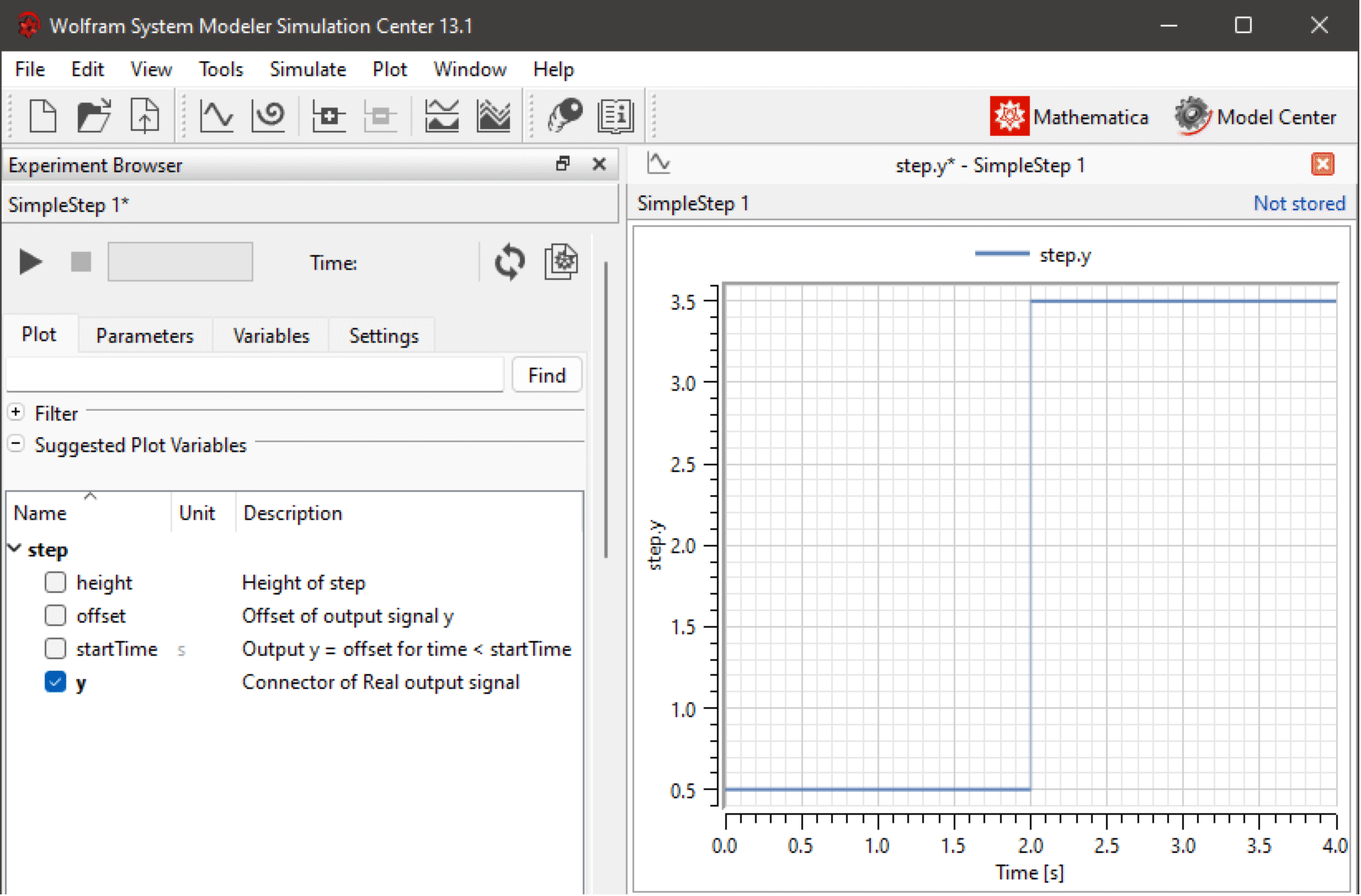
Although this does not look very useful yet, it still perfectly serves as a standalone model that one can simulate. This is going to be the first brick upon which you will build a simple model. Now proceed and simulate the model by clicking the Run button or pressing Ctrl+Shift+3. Once Simulation Center shows up, select the y variable to plot it as follows.
The plot of y as a function of time shown in Simulation Center.
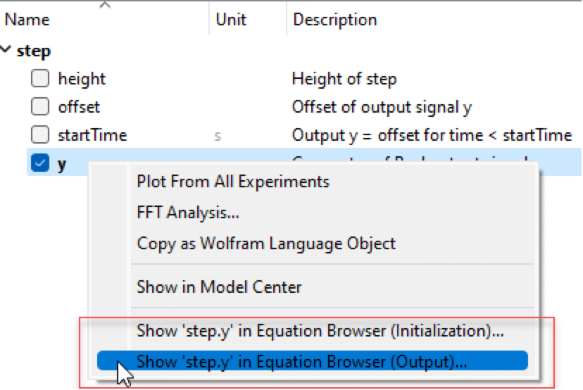
As expected from the initial values set for the parameters of the Step component, the value of y is 0.5 until 2 seconds and it jumps to 3.5 afterward. Now to open the Equation Browser, you have two options. You can either press Ctrl+3 or right-click the y parameter and select one of the menu items that point to the Equation Browser in the popup menu, as shown.
The popup menu items corresponding to Equation Browser.
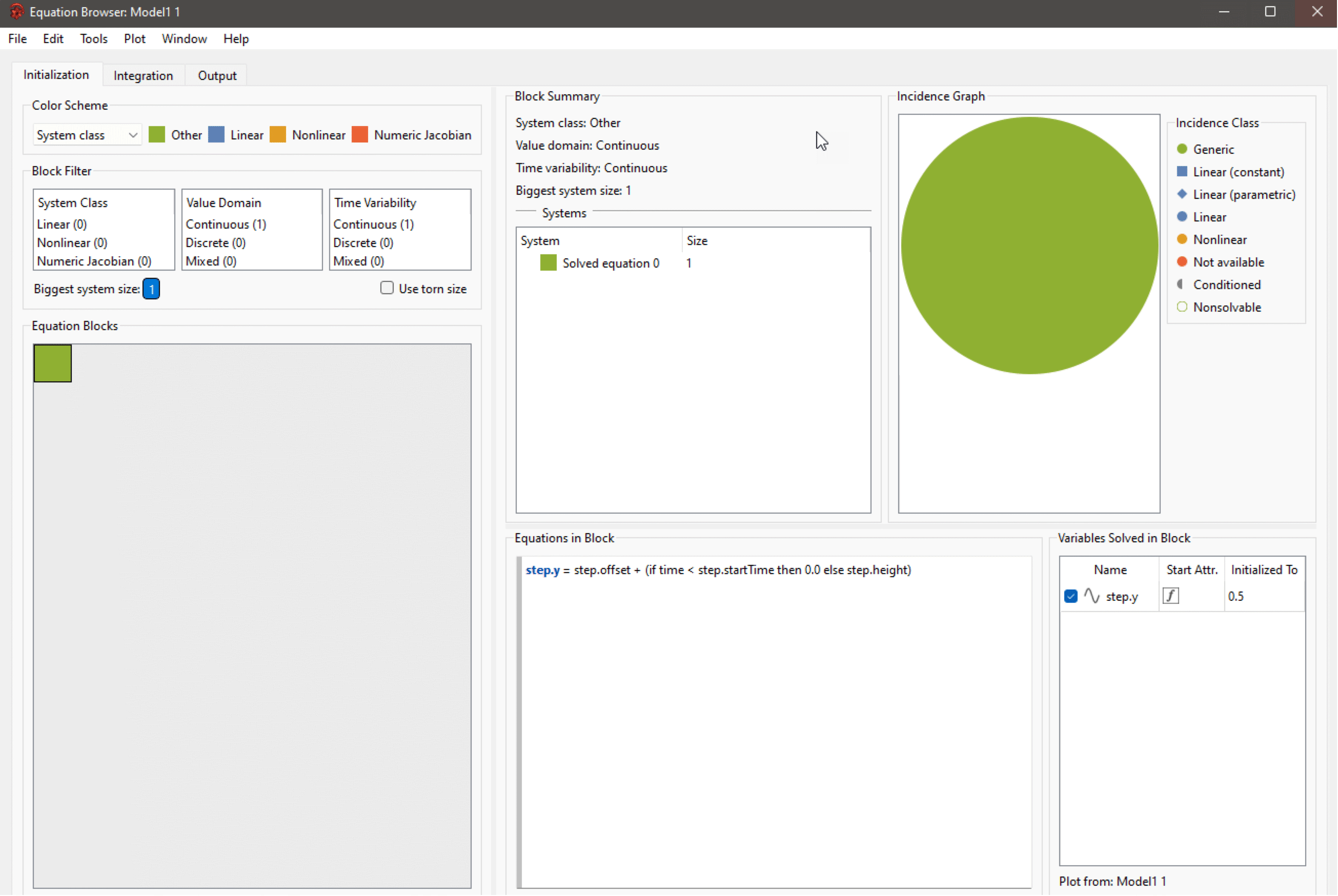
If you click the last item of the popup menu (which ends in Output) or use the keyboard shortcut keys, you get the Equation Browser, as follows.
You are now in the Output tab of the Equation Browser. As shown in the bottom-left panel, there is only one equation block. This block consists of a single equation system, which consists of a single equation (shown in the bottom-middle panel). Therefore, the size of the system and the biggest system size is 1. Since the only equation you see contains a simple if expression, it has been shown in green. This means there is nothing complex (nonlinear or numerical Jacobian) about it. This is good news! It is important to mention that it is not always possible to keep everything green or blue and entirely circumvent nonlinear equation systems or numeric Jacobians. Many models naturally bring such nonlinear equations into play, by design. However, you should try and work your way around such systems if possible.
The variables for which the equation system has been solved in the block are shown on the bottom-right panel. In this case, there is only y (step.y) which has been initially set to 0.5. The icon designated by the letter A and the corresponding red arrow states that y has been initialized according to a function or condition, i.e. the if expression in this case. In other words, it means System Modeler ignores (or overrides) the values you set to initialize such variables. In a separate tutorial specific to the initialization problem (Troubleshooting Model Initialization), you will learn about the implications and advantages of such behavior. Icon B indicates that y is continuous in time.
Now add a Product component and connect it to step as follows. Alternatively, you can open the StepSquared example.
Diagram view of the StepSquared model including Step and Product components.
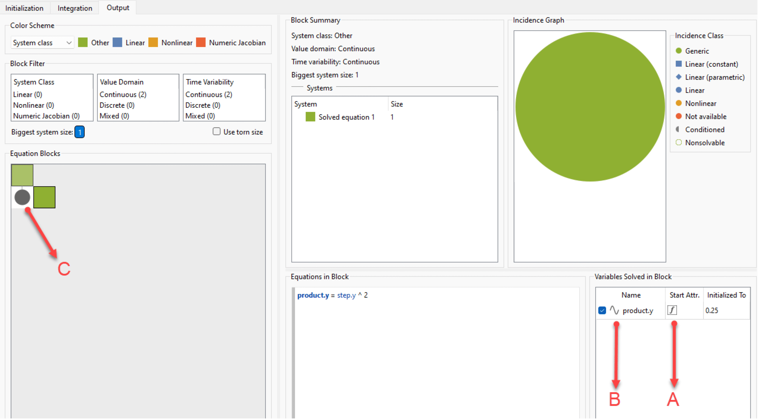
Simulate the model and open the Equation Browser. As shown, you see that there are now two blocks lying on a diagonal. The first block (upper-left corner) has remained as same as the previous step. The second block includes one equation that simply squares the given input. Icon C signifies that the output/result of the first block (step.y) has been used in or fed into the second block. Interestingly enough, System Modeler has automatically picked up on the fact that both inputs of the product component come from the same source and are equal, hence the equation includes exponentiation (step.y^2) instead of multiplication. Great!
Equation blocks of the model including Step and Product components.
Identifying Potential Bottlenecks
Now you will add one more level of complexity, namely a Feedback component. The diagram of the model looks like the following.
Diagram view of the Feedback model.
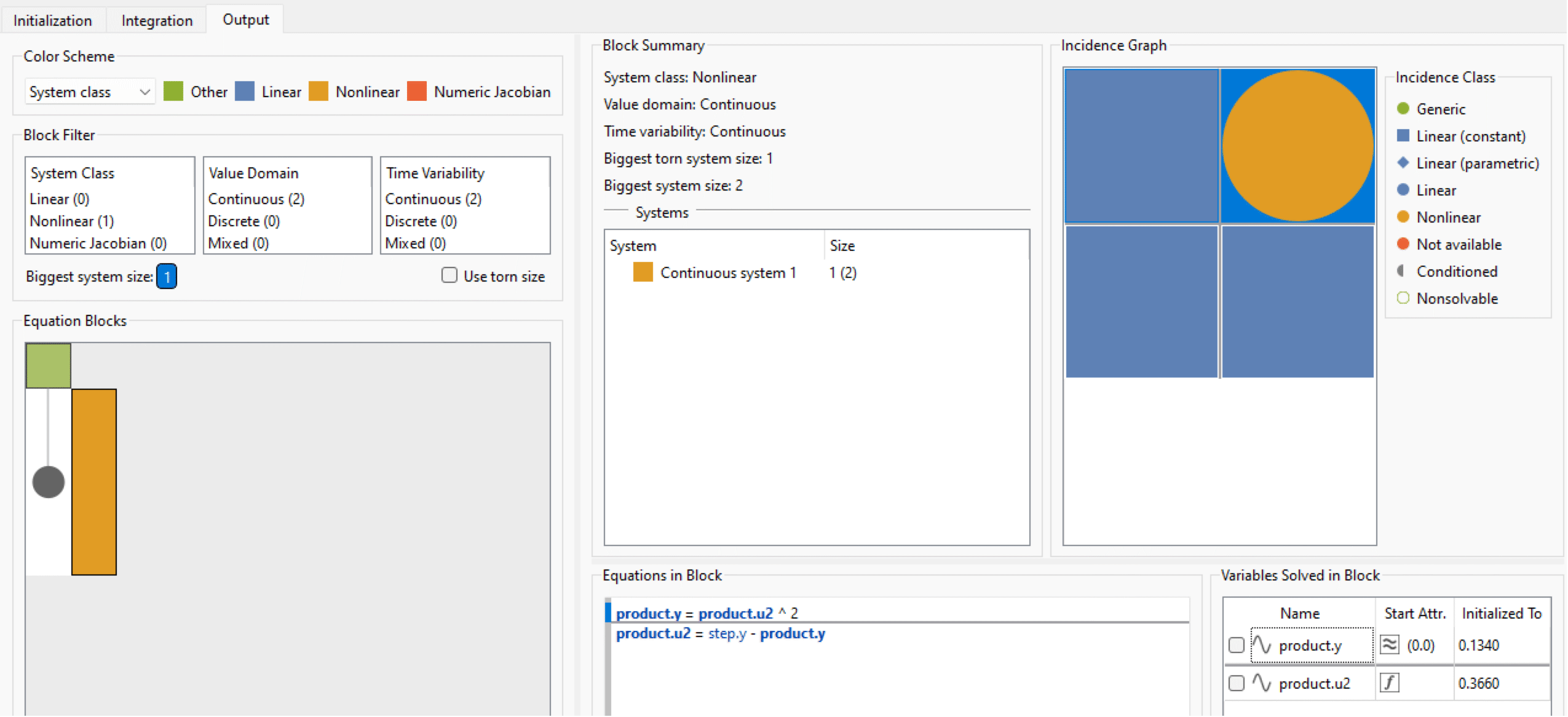
If you now simulate the Feedback model and inspect the Equation Browser, you will see a nonlinear equation system shown in orange. As mentioned earlier, this is not generally desirable and if possible, you should work your way around such systems.
Equation blocks of the model after the addition of a Feedback component.
In addition to the nonlinear equation system, one can observe that the Incidence Graph (top-right panel) is no longer composed of a single green circle as in previous steps, but rather it is now a 22 matrix. The Incidence Graph categorizes variables in each equation in terms of the so-called incidence classes.
One can think of this Incidence Graph as a more detailed or enriched representation of equation systems. Each row of the graph corresponds to one equation. There are two equations in the orange block, hence two rows in the Incidence Graph. The columns of the graph represent the variables in the equation. The color scheme determines the incidence class, where the green side of the spectrum is, as you might have guessed, preferable! By clicking or hovering over the orange circle, you can see that the nonlinearity is due to product.u2. This has occurred as a result of the feedback component, which makes the input of the product (product.u2) component depend upon its output (product.y), making a loop or cyclic dependency between input and output.
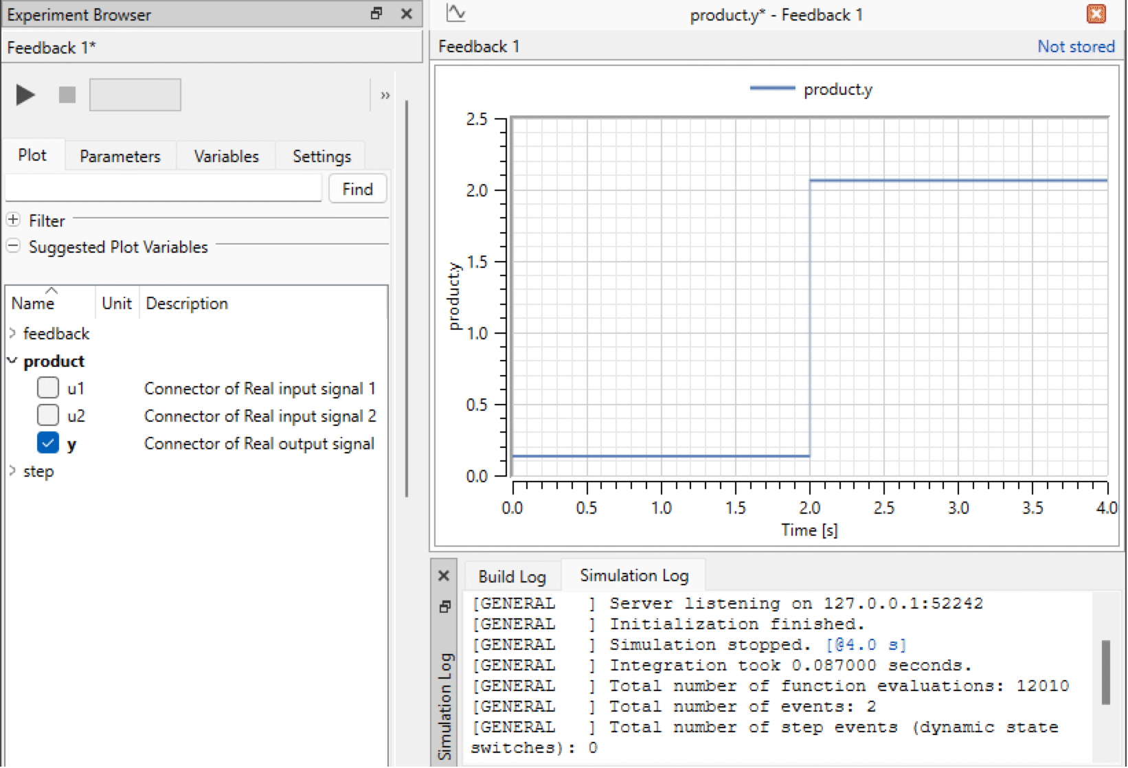
It is worth plotting the output of the product component. Note that there are no dynamics in the feedback loop, hence the output is a static function of step.y, as shown.
The simulation log of the model shown in Simulation Center.
Lowpass Filter to the Rescue
So far, you have identified that the existence of the aforementioned nonlinear equation system is due to the cyclic dependency of the input on the output and vice versa. If you can break this loop and decouple input from output in some way, you should be able to address this issue. Obviously, the resolution is not unique and one can think of different methods to decouple input and output of the product component. For example, this can be achieved by adding a filter such as LowpassButterworth between feedback and product. Leave the parameters of the filter component to their default values and simulate the FilteredFeedback model.
Diagram view of the FilteredFeedback model with the addition of the filter component.
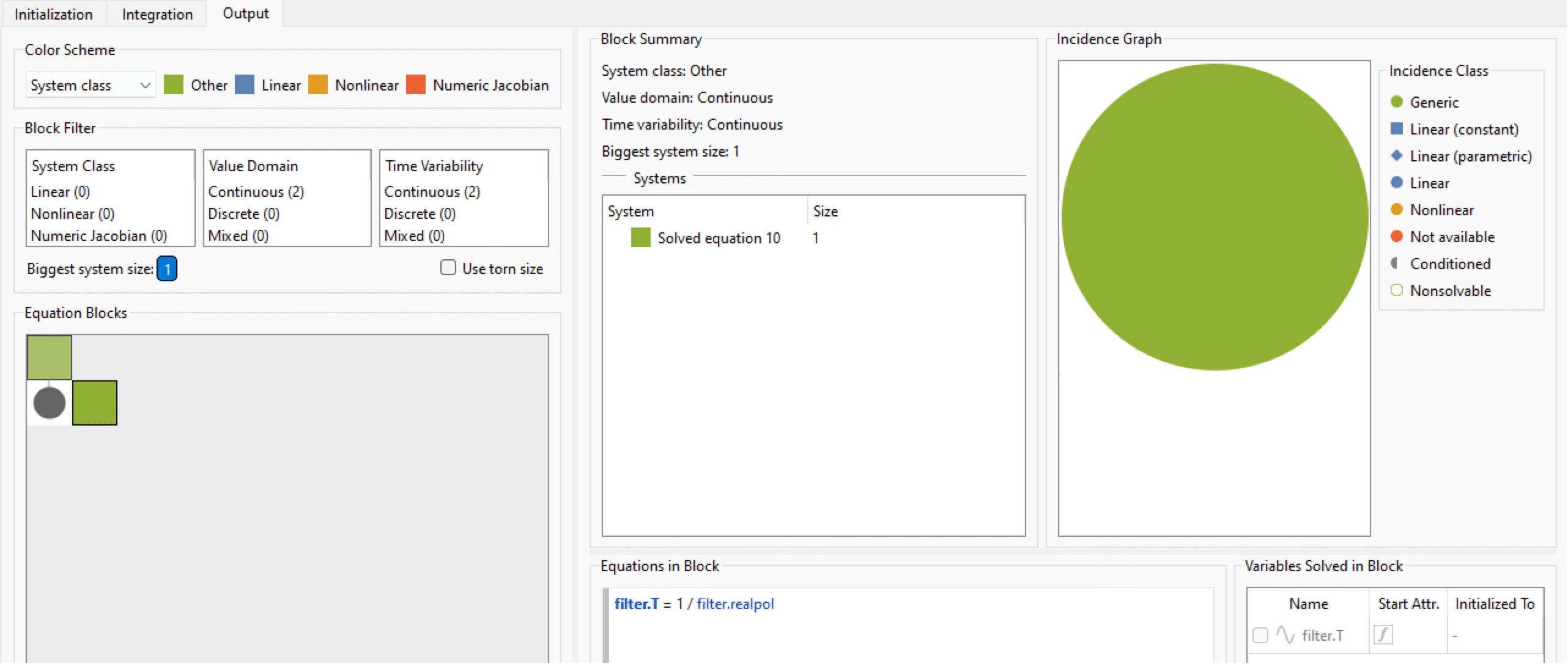
An inspection of the Equation Browser now reveals that the nonlinear equation system has miraculously disappeared and you are back to all green!
Equation blocks of the model after the addition of the filter component.
The magic behind the scene is that the filter breaks the loop and this way decouples the system, i.e. divide and conquer.
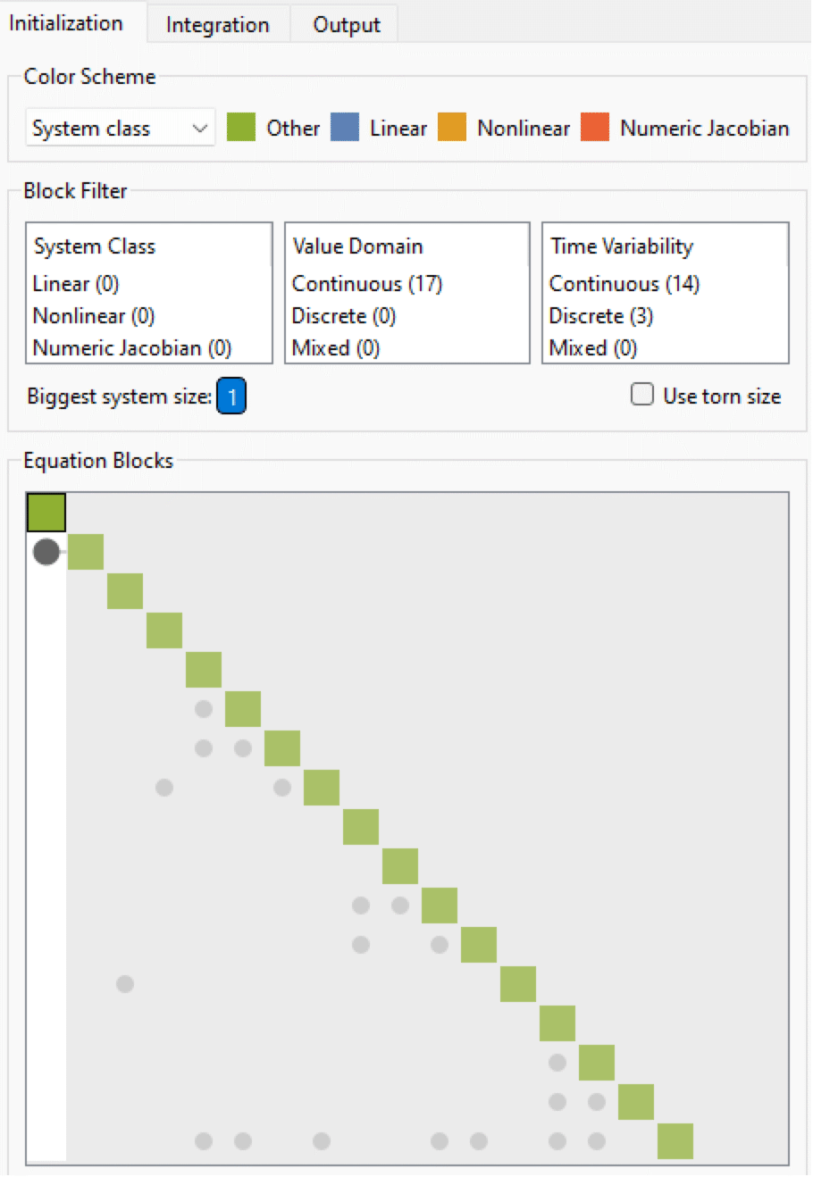
Having restored the model to a green state, you can further investigate the possible consequences of the addition of such a filter in the Initialization tab. One can see that the initialization problem is no longer as simple as before, yet it is all green!
Equation blocks of the model in the Initialization tab.
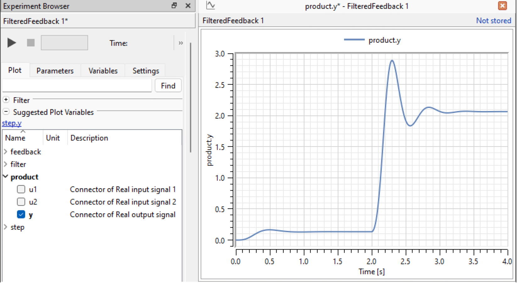
Moreover, the output signal now is showing some initial oscillations before leveling off to a constant value, in contrast to the pure staircase response from the step component you had earlier.
Output signal after the introduction of the Filter component.
Sum It All Up
This simple example was an introduction to Equation Browser and a few of its use cases. It demonstrated how one could simply split nonlinear blocks into linear ones. In particular, by introducing a filter, you managed to divide and conquer. For this small example, it was not necessary to look into the performance of the models, as the addition of the filter made no significant difference in the runtime of the simulation.
Breaking the loop and eliminating the nonlinear block did not come entirely cost free! This was achieved at the expense of: (1) making the initialization problem slightly more complex, albeit still totally linear; and (2) introducing some artifacts (oscillations) to the output signal during the early simulation time steps.
The focus of this example was on the response of the system after reaching the equilibrium, i.e. a constant value. In some cases, such alterations to the initialization and the system response might not be desirable. This demands the careful inspection of the modeler, not to utilize Equation Browser and such resolutions as a blind shot.


