WOLFRAM SYSTEM MODELER
BallAndBeamPIDModel of a ball and beam setup controlled by a PID-controller |
|
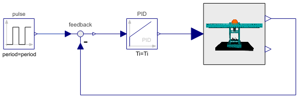
Diagram
Wolfram Language
In[1]:=
SystemModel["EducationExamples.Physics.BallAndBeam.BallAndBeamPID"]
Out[1]:=
Information
This model studies a ball rolling on top of a beam. The ball translational acceleration will be dependent on how the beam is angled. This example studies two different control schemes, the PID regulator and the LQ regulator, which can be used to control the position of the ball along the beam, using the beam angle as input.
Dynamics
Gravity acts on the ball, providing a downward force that is proportional to the mass of the object. When the beam is perpendicular to the gravitational force, parallell to the ground, the normal force exactly cancels out the gravitational force, and no acceleration is applied to the ball.
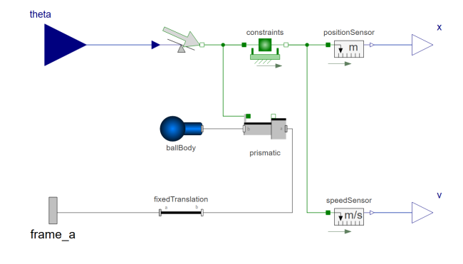
When the beam is angled, the ball will start to roll. The force now acting on the ball is proportional to the angle; a steeper angle will give the ball a higher acceleration.
The ball is assumed to roll ideally, without slipping. It is also assumed that the ball rolling on the beam is similar to a table tennis ball, with a thin outer shell and hollow on the inside.
Simulation
Simulate the model by clicking the Simulate button: 
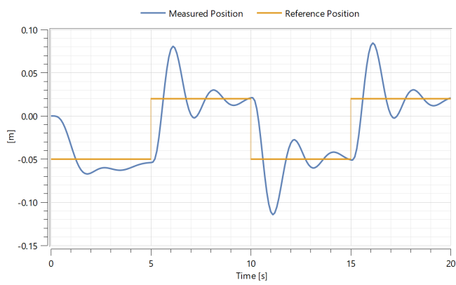
Plot the results
Explore how the actual ball position differs from the reference ball position. Do this by plotting the variables x and y. The first variable describes the reference position and the latter describes the measured position. This plot will be displayed immediately upon simulation.
You should now see the following plot:
Visualize
Multibody systems have automatic visualizers to show what a real-world system would look like.
In this example, custom CAD models have been loaded to better represent the system. To see a 3D representation of the system, follow the steps below:
Click the Animation button: 
Use your mouse or trackpad to drag the animation to a good angle and zoom in with your scroll wheel or by using the trackpad. Then click the Play button: 

In order to get the full experience of this example, you need a desktop Wolfram Language product. A free trial download is available at www.wolfram.com/mathematica/trial/
For the full example, open the accompanying notebook BallAndBeam.nb.
Parameters (6)
| amplitude |
Value: 0.07 Type: Length (m) Description: Amplitude of the reference pulse |
|---|---|
| offset |
Value: -0.05 Type: Length (m) Description: Offset of the reference pulse |
| period |
Value: 10 Type: Time (s) Description: Period of the reference pulse |
| k |
Value: 0.509581 Type: Real Description: Gain (PID.k) |
| Ti |
Value: 2.12121 Type: Time (s) Description: Time Constant of Integrator (PID.Ti) |
| Td |
Value: 0.942856 Type: Time (s) Description: Time Constant of Derivative block (PID.Td) |
Connectors (4)
| x |
Type: RealOutput Description: Ball position along the beam |
|
|---|---|---|
| v |
Type: RealOutput Description: Ball velocity along the beam |
|
| y |
Type: RealOutput Description: Reference signal |
|
| u |
Type: RealOutput Description: Input variable for the servo |
Components (4)
| ballAndBeam |
Type: BallAndBeamModel Description: Ball, beam and base assembly |
|
|---|---|---|
| feedback |
Type: Feedback Description: Output difference between commanded and feedback input |
|
| pulse |
Type: Pulse Description: Generate pulse signal of type Real |
|
| PID |
Type: PID Description: PID controller in additive description form |