

InitializePDECoefficients
InitializePDECoefficients[vd,sd,rules]
initializes the coefficients specified by rules in accordance with variable data vd and solution data sd to generate a PDECoefficientData object.
更多信息和选项
- The coefficients are assumed to come from a second-order system of
 PDEs in
  space dimensions of the form:
 - In InitializePDECoefficients[vd,sd,rules], the rules should be of the form name->coefficient. The possible coefficient names are:
-
"LoadCoefficients" {{f1},{f2},…}  is a scalar
"LoadDerivativeCoefficients" {{γ1},{γ2},…}  is a vector of length
"DiffusionCoefficients" {{-c11,-c12,…},{-c21,-c22,…},…}  may be specified as scalars, diagonal vectors of length
  , or
, or  ×
× matrices
"ConservativeConvectionCoefficients" {{-α11,-α12,…},{-α21,-α22,…},…}  is a vector of length
"ConvectionCoefficients" {{β11,β12,…},{β21,β22,…},…}  is a vector of length
"ReactionCoefficients" {{a11,a12,…},{a21,a22,…},…}  is a scalar
"DampingCoefficients" {{d11,d12,…},{d21,d22,…},…}  is a scalar
"MassCoefficients" {{m11,m12,…},{m21,m22,…},…}  is a scalar
 - If a rule is not specified for any of these coefficient names, the coefficients of that type are all assumed to be 0.
- Transient system of PDEs may be specified up through second order based on the form:
- NDSolve reduces transient systems so that they are first order in time.
- The coefficients can be functions of space, time, parameters, dependent variables and first order derivatives of dependent variables.
- Variable data vd and solution data sd are corresponding lists of variables and values. Templates for vd and sd may be generated using NDSolve`VariableData and NDSolve`SolutionData, and components may be set using NDSolve`SetSolutionDataComponent.
- InitializePDECoefficients verifies and optimizes the coefficients in accordance with variable data vd and solution data sd.
- The "Space" component of vd and sd should be set to the spatial variables and the spatial mesh represented as a NumericalRegion object, respectively.
- The "DependentVariables" component of vd should be a list of dependent variable name symbols without arguments.
- For time-dependent problems, the "Time" component of vd and sd should be set to the temporal variable and the initial time, respectively.
- For nonlinear problems, the "DependentVariables" component of sd should be set to the initial seedings for the dependent variables.
- For parametric problems, the "Parameters" component of vd and sd should be set to the parametric variables and the initial parametric values, respectively.
- InitializePDECoefficients has the following options:
-
"VerificationData" Automatic specify PDE coefficient verification data - Options given to InitializePDECoefficients can be given to NDSolve by specifying "InitializePDECoefficientsOptions". »
- Setting the option from NDSolve and related functions is explained in NDSolve Finite Element Options.


范例
打开所有单元 关闭所有单元基本范例 (2)
Load the finite element package:
Set up a NumericalRegion:
Set up variable and solution data:


Scope (6)
Coefficients can be functions:
Coefficients can be interpolation functions:
Coefficients can be nonlinear:
If the input for "DiffusionCoefficient" is a vector, it is interpreted as the diagonal of the requested input matrix:
If the input for "DiffusionCoefficient" is a scalar, the scalar is put in all places of the diagonal of the requested matrix:
Options (1)
"VerificationData" (1)
The PDE coefficients that are given to InitializePDECoefficients are verified so that they evaluate to numeric input:

The verification is done by finding a test coordinate that lies within the NumericalRegion. It may, however, happen that the automatically chosen test coordinate or test ElementMarker are at a singularity:

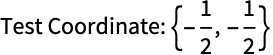

Overwriting the automatic finding of the verification data can be done with the "VerificationData" option:

Additionally, the automatic ElementMarker can be changed:

For nonlinear problems, the verification data for the dependents and the derivative of the dependents can be modified with "DependentVariables" and "DependentVariablesDerivative", respectively:

Change the test value for the dependent variable to be 1 and not 0 from the initial condition:
Change the test value of the derivative of the dependent variable to the vector {1,1}. The components of the vector are the values of the derivative in each space direction. Currently, a default 0.1 is used:
Applications (5)
Specify a Laplace equation  over a disk with Dirichlet and Neumann conditions
  for
for  and
and  for
for  :
:
Inspect the diffusion coefficients:
Discretize, solve, interpolate and visualize the solution:
The "LoadCoefficients" coefficient is used by NIntegrate to integrate over a region:
Use NIntegrate to verify the result:
A "ReactionCoefficients" of  can be used to evaluate a function, for example,
  over a region:
Visualize the evaluated function:
A "ReactionCoefficients" of  in combination with a "LoadCoefficients" can be used to scale a function, for example,
  over a region by a factor of
  :
:
Visualize the scaled evaluated function:
A "ReactionCoefficients" in combination with a "LoadDerivativeCoefficients" can be used to interpolate the derivative of a function over a region:
Visualize the difference between the numerical approximation and the exact derivative:
Properties & Relations (2)
Options given to InitializePDECoefficients can be given to NDSolve by specifying "InitializePDECoefficientOptions":

Specify "VerificationData" to pass a coordinate that is not at a singularity:
Convert a Poisson equation  into coefficients:
Use GetInactivePDE to create an inactive version of the input:
Possible Issues (1)
Typically, NDSolve will detect if coefficients do not evaluate to numeric quantities with the correct dimensions and warn about that:

To verify that the coefficients given are adequate for each operator, the coefficients undergo a test evaluation using the initial point in time and a coordinate from the region. If the combination of the coefficient and the used values cancel out, NDSolve cannot detect if a coefficient has not been specified. NDSolve will then give a message that it was not able to compute the elements contributed by a specific operator:




In the preceding case, evaluating the load operator at t=0 and x=-π will let the load operator vanish, and NDSolve cannot detect that k has not been specified:
文本
Wolfram Research (2014),InitializePDECoefficients,Wolfram 语言函数,https://reference.wolfram.com/language/FEMDocumentation/ref/InitializePDECoefficients.html (更新于 2020 年).
CMS
Wolfram 语言. 2014. "InitializePDECoefficients." Wolfram 语言与系统参考资料中心. Wolfram Research. 最新版本 2020. https://reference.wolfram.com/language/FEMDocumentation/ref/InitializePDECoefficients.html.
APA
Wolfram 语言. (2014). InitializePDECoefficients. Wolfram 语言与系统参考资料中心. 追溯自 https://reference.wolfram.com/language/FEMDocumentation/ref/InitializePDECoefficients.html 年