Nonlinear Finite Element Method Verification Tests
This notebook contains tests that verify that the nonlinear Finite Element method works as expected. To run all tests, SelectAll and press Shift+Enter. The results will then be in the section Test Result Inspection.
Differential equations in tests are typically given in inactive form. In some cases, an inactive form of a differential equation is the only way to set a specific differential equation. The exact details of when an inactive equation is used are explained in the Finite Element Method Usage Tips tutorial. The sections about Formal Partial Differential Equations and NeumannValue and Formal Partial Differential Equations are particularly relevant. In the test suite, most tests would not strictly need an inactive form, but they are present so that the parsing of the equations can also be tested.
Note that these tests can also serve as a basis for developing your own differential equation models. As such, the tests are grouped into stationary (time-independent) and transient (time-dependent) tests. The next level of grouping is in the number of equations. Either a single equation or a coupled equation is considered. In those categories, one- and two-dimensional tests can be found. The fact that no three-dimensional tests are present is due to implementation of the finite element code. The code base for all dimensions is the same, and not much benefit would come from including three-dimensional tests.
Some cells in the actual tests are not evaluatable. These are mainly cells that contain a symbolic derivation and would take additional runtime and consume memory. If an actual analytical solution exists, it is given as a function. The derivation is there for inspection. To make these cells evaluatable, select the cells in question and choose Cell ▶ Cell Properties and make sure "Evaluatable" is ticked.
The individual subtest also needs to be evaluated in order to work as intended.
Needs["NDSolve`FEM`"]
Needs["MUnit`"]sopts = {"FiniteElement"};
topts = {"PDEDiscretization" -> {"MethodOfLines", "SpatialDiscretization" -> "FiniteElement"}};$HistoryLength = 0;Stationary Tests
This section contains examples of stationary (non-time-dependent) nonlinear partial differential equations.
1D Single Equation
This section contains examples of ordinary nonlinear differential equations with one equation. Ordinary differential equations with one independent variable are a special case of partial differential equations that usually deal with more than one independent variable.
Diffusion—FEM-NL-Stationary-1D-Single-Diffusion-0001
Test Reference:
[1], chapter 7, page 341.
op = Inactive[Div][{{-u[x] ^ 2}}. Inactive[Grad][u[x], {x}], {x}] - 4ares = Function[x, (-6x ^ 2 + 18x + 1) ^ (1 / 3)]bcs = {DirichletCondition[u[x] == 1., x == 0], NeumannValue[2., x == 1]}region = Line[{{0}, {1}}]Test 1:
VerificationTest[
	nlfun = NDSolveValue[{op == bcs[[2]], bcs[[1]]}, u, Element[{x}, region], Method -> sopts, InitialSeeding -> {u[x] == 1}];
	Norm[Table[nlfun[x] - ares[x], {x, 0, 1, 0.1}]] < 10 ^ -9,
	True,
	TestID -> "FEM-NL-Stationary-1D-Single-Diffusion-0001-A"
	]
Test 2:
VerificationTest[
	aeqn = Activate[op - bcs[[2]] == 0];
	anlfun = NDSolveValue[{aeqn, bcs[[1]]}, u, Element[{x}, region], Method -> sopts, InitialSeeding -> {u[x] == 1}];
	Norm[Table[anlfun[x] - ares[x], {x, 0, 1, 0.1}]] < 10 ^ -9,
	True,
	TestID -> "FEM-NL-Stationary-1D-Single-Diffusion-0001-B"
	]
Test 3:
VerificationTest[
	vd = NDSolve`VariableData[{"Dependent", "Space"} -> {{u}, {x}}];
	nr = ToNumericalRegion[region];
	sd = NDSolve`SolutionData[{"Dependent", "Space"} -> {{1}, nr}];
	md = InitializePDEMethodData[vd, sd];
	ibcs = InitializeBoundaryConditions[vd, sd, {bcs}];
	pdec = InitializePDECoefficients[vd, sd
	, "DiffusionCoefficients" -> {{{{-u[x] ^ 2}}}}
	, "LoadCoefficients" -> {{4}}
	];
	j = e = s = 0;
	sdNew = PDESolve[pdec, ibcs, vd, sd, md,
	"FindRootOptions" -> {Jacobian -> {Automatic, EvaluationMonitor :> j++}, EvaluationMonitor :> e++, StepMonitor :> s++}
	];
	{eif} = ProcessPDESolutions[md, sdNew];
{Norm[Table[eif[x] - ares[x], {x, 0, 1, 0.1}]] < 10 ^ -9, e == 11, s == 10, j == 3}
	,
	{True, True, True, True},
	{TestID -> "FEM-NL-Stationary-1D-Single-Diffusion-0001-C"}
]Diffusion—FEM-NL-Stationary-1D-Single-Diffusion-0002
Test Reference:
[4], page 38
The right-hand-side f will be computed from the analytical solution.
op = Inactive[Div][{{-q[u[x]]}}. Inactive[Grad][u[x], {x}], {x}]params = {q[u_] -> ((1 + u) ^ m), m -> 2}ares = Function[{x}, Evaluate[((2 ^ (m + 1) - 1) * x + 1) ^ (1 / (m + 1)) - 1 //. params]]f = Activate[op //. params] /. u -> aresbcs = {DirichletCondition[u[x] == 0., x == 0], DirichletCondition[u[x] == 1., x == 1]}region = Line[{{0}, {1}}]Test 1:
VerificationTest[
	nlfun = NDSolveValue[{op == f, bcs} //. params, u, Element[{x}, region], Method -> sopts, InitialSeeding -> {u[x] == x}];
	Norm[Table[nlfun[x] - ares[x], {x, 0, 1, 0.1}]] < 10 ^ -8,
	True,
	TestID -> "FEM-NL-Stationary-1D-Single-Diffusion-0002-A"
	]
Test 2:
VerificationTest[
	aeqn = Activate[op == f //. params];
	anlfun = NDSolveValue[{aeqn, bcs}, u, Element[{x}, region], Method -> sopts, InitialSeeding -> {u[x] == x}];
	Norm[Table[anlfun[x] - ares[x], {x, 0, 1, 0.1}]] < 10 ^ -8,
	True,
	TestID -> "FEM-NL-Stationary-1D-Single-Diffusion-0002-B"
	]
Test 3:
VerificationTest[
	vd = NDSolve`VariableData[{"Dependent", "Space"} -> {{u}, {x}}];
	mesh = ToElementMesh[region, "MeshElementBlocks" -> 3];
	nr = ToNumericalRegion[mesh];
	sd = NDSolve`SolutionData[{"Dependent", "Space"} -> {{x}, nr}];
	md = InitializePDEMethodData[vd, sd];
	ibcs = InitializeBoundaryConditions[vd, sd, {bcs}];
	pdec = InitializePDECoefficients[vd, sd
	, "DiffusionCoefficients" -> {{{{-q[u[x]]}}}} //. params
	, "LoadCoefficients" -> {{f}}
	];
	sdNew = PDESolve[pdec, ibcs, vd, sd, md];
	{eif} = ProcessPDESolutions[md, sdNew];
	{Norm[Table[eif[x] - ares[x], {x, 0, 1, 0.1}]] < 10 ^ -8, Length[mesh["MeshElements"]]}
	,
	{True, 3},
	{TestID -> "FEM-NL-Stationary-1D-Single-Diffusion-0002-C"}
]Convection—FEM-NL-Stationary-1D-Single-Convection-0001
Test Reference:
[2], problems: 3.7, page 83.
op = Inactive[Div][{{-1}}. Inactive[Grad][u[x], {x}], {x}] - 2u[x] * D[u[x], x]ares = Function[x, 1 / (1 + x)]bcs = {DirichletCondition[u[x] == 1, x == 0], DirichletCondition[u[x] == 1 / 2, x == 1]}region = Line[{{0}, {1}}]Test 1:
VerificationTest[
	nlfun = NDSolveValue[{op == 0, bcs}, u, Element[{x}, region], Method -> "FiniteElement", InitialSeeding -> {u[x] == 1}];
	Norm[Table[nlfun[x] - ares[x], {x, 0, 1, 0.1}]] < 10 ^ -7,
	True,
	TestID -> "FEM-NL-Stationary-1D-Single-Convection-0001-A"
	]
Test 2:
VerificationTest[
	anlfun = NDSolveValue[{Activate[op == 0], bcs}, u, Element[{x}, region], Method -> "FiniteElement", InitialSeeding -> {u[x] == 1}];
	Norm[Table[anlfun[x] - ares[x], {x, 0, 1, 0.1}]] < 10 ^ -7,
	True,
	TestID -> "FEM-NL-Stationary-1D-Single-Convection-0001-B"
	]
Test 3:
VerificationTest[
	nr = ToNumericalRegion[region];vd = NDSolve`VariableData[{"Dependent", "Space"} -> {{u}, {x}}];sd = NDSolve`SolutionData[{"Dependent", "Space"} -> {{1}, nr}];
	md = InitializePDEMethodData[vd, sd];ibcs = InitializeBoundaryConditions[vd, sd, {bcs}];
	pdec = InitializePDECoefficients[vd, sd
	, "DiffusionCoefficients" -> {{{{-1}}}}
	, "ConvectionCoefficients" -> {{{{-2u[x]}}}}
	];
	j = e = s = 0;
	sdNew = PDESolve[pdec, ibcs, vd, sd, md,
	"FindRootOptions" -> {Jacobian -> {Automatic, EvaluationMonitor :> j++}, EvaluationMonitor :> e++, StepMonitor :> s++}
	];
	{eif} = ProcessPDESolutions[md, sdNew];
{Norm[Table[eif[x] - ares[x], {x, 0, 1, 0.1}]] < 10 ^ -7, e == 10, s == 9, j == 1}
	,
	{True, True, True, True},
	{TestID -> "FEM-NL-Stationary-1D-Single-Convection-0001-C"}
]Convection—FEM-NL-Stationary-1D-Single-Convection-0002
Test Reference:
op = Inactive[Div][{{1}}. Inactive[Grad][u[x], {x}], {x}] + u[x] * D[u[x], x] - u[x] - Exp[2 x]ares = Function[x, Exp[x]]Activate[op == 0] /. u -> ares//Simplifybcs = {NeumannValue[2 - u[x], x == 0], DirichletCondition[u[x] == E, x == 1]}region = Line[{{0}, {1}}]Test 1:
VerificationTest[
	nlfun = NDSolveValue[{op == bcs[[1]], bcs[[2]]}, u, Element[{x}, region], Method -> "FiniteElement"];
	Norm[Table[nlfun[x] - ares[x], {x, 0, 1, 0.1}]] < 10 ^ -6,
	True,
	TestID -> "FEM-NL-Stationary-1D-Single-Convection-0002-A"
	]
Test 2:
VerificationTest[
	anlfun = NDSolveValue[{Activate[op == bcs[[1]]], bcs[[2]]}, u, Element[{x}, region], Method -> "FiniteElement"];
	Norm[Table[anlfun[x] - ares[x], {x, 0, 1, 0.1}]] < 10 ^ -6,
	True,
	TestID -> "FEM-NL-Stationary-1D-Single-Convection-0002-B"
	]
Test 3:
VerificationTest[
	nr = ToNumericalRegion[region];vd = NDSolve`VariableData[{"Dependent", "Space"} -> {{u}, {x}}];sd = NDSolve`SolutionData[{"Dependent", "Space"} -> {{1}, nr}];
	md = InitializePDEMethodData[vd, sd];ibcs = InitializeBoundaryConditions[vd, sd, {bcs}];
	pdec = InitializePDECoefficients[vd, sd
	, "DiffusionCoefficients" -> {{{{1}}}}
	, "ConvectionCoefficients" -> {{{{u[x]}}}}
	, "ReactionCoefficients" -> {{-1}}
	, "LoadCoefficients" -> {{Exp[2 x]}}
	];
	j = e = s = 0;
	sdNew = PDESolve[pdec, ibcs, vd, sd, md,
	"FindRootOptions" -> {Jacobian -> {Automatic, EvaluationMonitor :> j++}, EvaluationMonitor :> e++, StepMonitor :> s++}
	];
	{eif} = ProcessPDESolutions[md, sdNew];
{Norm[Table[eif[x] - ares[x], {x, 0, 1, 0.1}]] < 10 ^ -6, e == 12, s == 11, j == 1}
	,
	{True, True, True, True},
	{TestID -> "FEM-NL-Stationary-1D-Single-Convection-0002-C"}
]Reaction—FEM-NL-Stationary-1D-Single-Reaction-0001
Test Reference:
[1], problem 7.1, page 383.
op = Inactive[Plus][Inactive[Div][{{-1}}. Inactive[Grad][u[x], {x}], {x}], u[x] ^ 3]bcs = {DirichletCondition[u[x] == 1 / 27, x == 0], NeumannValue[5 / 3, x == 2]}region = Line[{{0}, {2}}]nres = NDSolveValue[{op == 0//Activate, u[0] == 1 / 27, u'[2] == 5 / 3}, u, {x, 0, 2}, Method -> "Shooting"]Test 1:
VerificationTest[
	nlfun = NDSolveValue[{op == bcs[[2]], bcs[[1]]}, u, Element[{x}, region], Method -> sopts, InitialSeeding -> {u[x] == 1}];
	Norm[Table[nlfun[x] - nres[x], {x, 0, 2, 0.1}]] < 10 ^ -5,
	True,
	TestID -> "FEM-NL-Stationary-1D-Single-Reaction-0001-A"
	]
Test 2:
VerificationTest[
	aeqn = Activate[op - bcs[[2]] == 0];anlfun = NDSolveValue[{aeqn, bcs[[1]]}, u, Element[{x}, region], Method -> sopts, InitialSeeding -> {u[x] == 1}];
	Norm[Table[anlfun[x] - nres[x], {x, 0, 1, 0.1}]] < 10 ^ -5,
	True,
	TestID -> "FEM-NL-Stationary-1D-Single-Reaction-0001-B"
	]
Test 3:
VerificationTest[
	vd = NDSolve`VariableData[{"Dependent", "Space"} -> {{u}, {x}}];
	nr = ToNumericalRegion[region];
	sd = NDSolve`SolutionData[{"Dependent", "Space"} -> {{1}, nr}];
	md = InitializePDEMethodData[vd, sd];
	ibcs = InitializeBoundaryConditions[vd, sd, {bcs}];
	pdec = InitializePDECoefficients[vd, sd
	, "DiffusionCoefficients" -> {{{{-1}}}}
	, "ReactionCoefficients" -> {{u[x] ^ 2}}
	];
	j = e = s = 0;
	sdNew = PDESolve[pdec, ibcs, vd, sd, md,
	"FindRootOptions" -> {Jacobian -> {Automatic, EvaluationMonitor :> j++}, EvaluationMonitor :> e++, StepMonitor :> s++}
	];
	{eif} = ProcessPDESolutions[md, sdNew];
{Norm[Table[eif[x] - nres[x], {x, 0, 1, 0.1}]] < 10 ^ -5, e == 11, s == 10, j == 1}
	,
	{True, True, True, True},
	{TestID -> "FEM-NL-Stationary-1D-Single-Reaction-0001-C"}
]Reaction—FEM-NL-Stationary-1D-Single-Reaction-0002
Test Reference:
[1], problem 7.3, page 384.
logTerm = (2u[x] - Log[x]) ^ 3;
op = Inactive[Plus][Inactive[Div][{{1}}. Inactive[Grad][u[x], {x}], {x}], -D[u[x], x], -logTerm]bcs = {DirichletCondition[u[x] == 1 / 2, x == 1], DirichletCondition[u[x] == 1 / 2 + Log[2], x == 2]}region = Line[{{1}, {2}}]nres = NDSolveValue[{op == 0//Activate, u[1] == 1 / 2, u[2] == 1 / 2 + Log[2]}, u, {x, 1, 2}]Test 1:
VerificationTest[
	nlfun = NDSolveValue[{op == 0, bcs}, u, Element[{x}, region], Method -> sopts, InitialSeeding -> {u[x] == 1}];
	Norm[Table[nlfun[x] - nres[x], {x, 1, 2, 0.1}]] < 10 ^ -6,
	True,
	TestID -> "FEM-NL-Stationary-1D-Single-Reaction-0002-A"
	]
Test 2:
VerificationTest[
	aeqn = Activate[op == 0];anlfun = NDSolveValue[{aeqn, bcs}, u, Element[{x}, region], Method -> sopts, InitialSeeding -> {u[x] == 1}];
	Norm[Table[anlfun[x] - nres[x], {x, 1, 2, 0.1}]] < 10 ^ -6,
	True,
	TestID -> "FEM-NL-Stationary-1D-Single-Reaction-0002-B"
	]
Test 3 & 4:
vd = NDSolve`VariableData[{"Dependent", "Space"} -> {{u}, {x}}];
nr = ToNumericalRegion[region];
sd = NDSolve`SolutionData[{"Dependent", "Space"} -> {{1}, nr}];
md = InitializePDEMethodData[vd, sd];
ibcs = InitializeBoundaryConditions[vd, sd, {bcs}];VerificationTest[
pdec = InitializePDECoefficients[vd, sd
, "DiffusionCoefficients" -> {{{{1}}}}
, "ConvectionCoefficients" -> {{{{-1}}}}
, "ReactionCoefficients" -> {{-6 Log[x] ^ 2 + 12 Log[x] u[x] - 8 u[x] ^ 2}}
, "LoadCoefficients" -> {{-Log[x] ^ 3}}
];
j = e = s = 0;
sdNew = PDESolve[pdec, ibcs, vd, sd, md,
"FindRootOptions" -> {Jacobian -> {Automatic, EvaluationMonitor :> j++}, EvaluationMonitor :> e++, StepMonitor :> s++}
];
{eif} = ProcessPDESolutions[md, sdNew];
{Norm[Table[eif[x] - nres[x], {x, 1, 2, 0.1}]] < 10 ^ -5, e == 11, s == 10, j == 1}
,
{True, True, True, True},
{TestID -> "FEM-NL-Stationary-1D-Single-Reaction-0002-C"}
]VerificationTest[
pdec = InitializePDECoefficients[vd, sd
, "DiffusionCoefficients" -> {{{{1}}}}
, "ConvectionCoefficients" -> {{{{-1}}}}
, "LoadCoefficients" -> {{logTerm}}
];
j = e = s = 0;
sdNew = PDESolve[pdec, ibcs, vd, sd, md,
"FindRootOptions" -> {Jacobian -> {Automatic, EvaluationMonitor :> j++}, EvaluationMonitor :> e++, StepMonitor :> s++}
];
{eif} = ProcessPDESolutions[md, sdNew];
{Norm[Table[eif[x] - nres[x], {x, 1, 2, 0.1}]] < 10 ^ -5, e == 11, s == 10, j == 1}
,
{True, True, True, True},
{TestID -> "FEM-NL-Stationary-1D-Single-Reaction-0002-D"}
]Reaction—FEM-NL-Stationary-1D-Single-Reaction-0003
Test Reference:
op = Inactive[Plus][Inactive[Div][{{-1}}. Inactive[Grad][u[x], {x}], {x}], u[x] ^ 2](*ares=DSolveValue[{op==0//Activate},u,x]/.{C[1]->1,C[2]->1}*)
ares = Function[{x}, 6^1 / 3 WeierstrassP[(x + 1) / 6^1 / 3, {0, 1}]]No boundary conditions are specified; they are deduced from the analytical solution.
bcs = {DirichletCondition[u[x] == ares[0.], x == 0], DirichletCondition[u[x] == ares[1.], x == 1]}The test uses an arbitrary region.
region = Line[{{0}, {1}}]Test 1:
VerificationTest[
	nlfun = NDSolveValue[{op == 0, bcs}, u, Element[{x}, region], Method -> sopts, InitialSeeding -> {u[x] == 1}];
	Norm[Table[nlfun[x] - ares[x], {x, 0, 1, 0.1}]] < 10 ^ -5,
	True,
	TestID -> "FEM-NL-Stationary-1D-Single-Reaction-0003-A"
	]
Test 2:
VerificationTest[
	aeqn = Activate[op == 0];anlfun = NDSolveValue[{aeqn, bcs}, u, Element[{x}, region], Method -> sopts, InitialSeeding -> {u[x] == 1}];
	Norm[Table[anlfun[x] - ares[x], {x, 0, 1, 0.1}]] < 10 ^ -5,
	True,
	TestID -> "FEM-NL-Stationary-1D-Single-Reaction-0003-B"
	]
Test 3 & 4:
vd = NDSolve`VariableData[{"Dependent", "Space"} -> {{u}, {x}}];
nr = ToNumericalRegion[region];
sd = NDSolve`SolutionData[{"Dependent", "Space"} -> {{1}, nr}];
md = InitializePDEMethodData[vd, sd];
ibcs = InitializeBoundaryConditions[vd, sd, {bcs}];VerificationTest[
pdec = InitializePDECoefficients[vd, sd
, "DiffusionCoefficients" -> {{{{-1}}}}
, "LoadCoefficients" -> {{-u[x] ^ 2}}
];
j = e = s = 0;
sdNew = PDESolve[pdec, ibcs, vd, sd, md,
"FindRootOptions" -> {Jacobian -> {Automatic, EvaluationMonitor :> j++}, EvaluationMonitor :> e++, StepMonitor :> s++}
];
{eif} = ProcessPDESolutions[md, sdNew];
{Norm[Table[eif[x] - ares[x], {x, 0, 1, 0.1}]] < 10 ^ -5, e == 10, s == 9, j == 1}
,
{True, True, True, True},
{TestID -> "FEM-NL-Stationary-1D-Single-Reaction-0003-C"}
]VerificationTest[
pdec = InitializePDECoefficients[vd, sd
, "DiffusionCoefficients" -> {{{{-1}}}}
, "ReactionCoefficients" -> {{u[x]}}
];
j = e = s = 0;
sdNew = PDESolve[pdec, ibcs, vd, sd, md,
"FindRootOptions" -> {Jacobian -> {Automatic, EvaluationMonitor :> j++}, EvaluationMonitor :> e++, StepMonitor :> s++}
];
{eif} = ProcessPDESolutions[md, sdNew];
{Norm[Table[eif[x] - ares[x], {x, 0, 1, 0.1}]] < 10 ^ -5, e == 10, s == 9, j == 1}
,
{True, True, True, True},
{TestID -> "FEM-NL-Stationary-1D-Single-Reaction-0003-D"}
]Reaction—FEM-NL-Stationary-1D-Single-Reaction-0004
Test Reference:
op = Inactive[Plus][Inactive[Div][{{-1}}. Inactive[Grad][u[x], {x}], {x}], I u[x] ^ 2](*ares=DSolveValue[{op==0//Activate},u,x]/.{C[1]->1,C[2]->1}*)
ares = Function[{x}, -(-1)^5 / 6 6^1 / 3 WeierstrassP[((-1)^1 / 6 (x + 1)/6^1 / 3), {0, 1}]]No boundary conditions are specified; they are deduced from the analytical solution.
bcs = {DirichletCondition[u[x] == ares[0.], x == 0], DirichletCondition[u[x] == ares[1.], x == 1]}The test uses an arbitrary region.
region = Line[{{0}, {1}}]Test 1:
VerificationTest[
	nlfun = NDSolveValue[{op == 0, bcs}, u, Element[{x}, region], Method -> sopts, InitialSeeding -> {u[x] == 1}];
	Norm[Table[nlfun[x] - ares[x], {x, 0, 1, 0.1}]] < 10 ^ -5,
	True,
	TestID -> "FEM-NL-Stationary-1D-Single-Reaction-0004-A"
	]
Test 2:
VerificationTest[
	aeqn = Activate[op == 0];anlfun = NDSolveValue[{aeqn, bcs}, u, Element[{x}, region], Method -> sopts, InitialSeeding -> {u[x] == 1}];
	Norm[Table[anlfun[x] - ares[x], {x, 0, 1, 0.1}]] < 10 ^ -5,
	True,
	TestID -> "FEM-NL-Stationary-1D-Single-Reaction-0004-B"
	]
Test 3 & 4:
vd = NDSolve`VariableData[{"Dependent", "Space"} -> {{u}, {x}}];
nr = ToNumericalRegion[region];
sd = NDSolve`SolutionData[{"Dependent", "Space"} -> {{1}, nr}];
md = InitializePDEMethodData[vd, sd];
ibcs = InitializeBoundaryConditions[vd, sd, {bcs}];VerificationTest[
pdec = InitializePDECoefficients[vd, sd
, "DiffusionCoefficients" -> {{{{-1}}}}
, "LoadCoefficients" -> {{-I u[x] ^ 2}}
];
j = e = s = 0;
sdNew = PDESolve[pdec, ibcs, vd, sd, md,
"FindRootOptions" -> {Jacobian -> {Automatic, EvaluationMonitor :> j++}, EvaluationMonitor :> e++, StepMonitor :> s++}
];
{eif} = ProcessPDESolutions[md, sdNew];
{Norm[Table[eif[x] - ares[x], {x, 0, 1, 0.1}]] < 10 ^ -5, e == 13, s == 11, j == 2}
,
{True, True, True, True},
{TestID -> "FEM-NL-Stationary-1D-Single-Reaction-0004-C"}
]VerificationTest[
pdec = InitializePDECoefficients[vd, sd
, "DiffusionCoefficients" -> {{{{-1}}}}
, "ReactionCoefficients" -> {{I u[x]}}
];
j = e = s = 0;
sdNew = PDESolve[pdec, ibcs, vd, sd, md,
"FindRootOptions" -> {Jacobian -> {Automatic, EvaluationMonitor :> j++}, EvaluationMonitor :> e++, StepMonitor :> s++}
];
{eif} = ProcessPDESolutions[md, sdNew];
{Norm[Table[eif[x] - ares[x], {x, 0, 1, 0.1}]] < 10 ^ -5, e == 13, s == 11, j == 2}
,
{True, True, True, True},
{TestID -> "FEM-NL-Stationary-1D-Single-Reaction-0004-D"}
]Load—FEM-NL-Stationary-1D-Single-Load-0001
Test Reference:
[3], Exact Solutions > Ordinary Differential Equations > Second-Order Nonlinear Ordinary Differential Equations; Equation 3.1.1; Autonomous equation.
op = Inactive[Div][{{1}}. Inactive[Grad][u[x], {x}], {x}] - Sin[u[x]]where C1 and C2 are arbitrary constants.
(*temp=Integrate[(C[1]+2*Integrate[Sin[u[x]],u[x]])^(-1/2),u[x]]==C[2]+x/.{C[1]->3,C[2]->3};
ares=Function[x,Evaluate[(u[x]/.Solve[temp,u[x]])[[1]]]]*)
ares = Function[x, 2 JacobiAmplitude[(3 + x/2), -4]]Activate[op == 0] /. u -> ares//SimplifyNo boundary conditions are specified; they are deduced from the analytical solution.
bcs = {DirichletCondition[u[x] == ares[0.], x == 0], DirichletCondition[u[x] == ares[1.], x == 1]}The test uses an arbitrary region.
region = Line[{{0}, {1}}]Test 1:
VerificationTest[
	nlfun = NDSolveValue[{op == 0, bcs}, u, Element[{x}, region], Method -> sopts, InitialSeeding -> {u[x] == 1}];
	Norm[Table[nlfun[x] - ares[x], {x, 0, 1, 0.1}]] < 10 ^ -9,
	True,
	TestID -> "FEM-NL-Stationary-1D-Single-Load-0001-A"
	]
Test 2:
VerificationTest[
	aeqn = Activate[op == 0];anlfun = NDSolveValue[{aeqn, bcs}, u, Element[{x}, region], Method -> sopts, InitialSeeding -> {u[x] == 1}];
	Norm[Table[anlfun[x] - ares[x], {x, 0, 1, 0.1}]] < 10 ^ -9,
	True,
	TestID -> "FEM-NL-Stationary-1D-Single-Load-0001-B"
	]
Test 3:
VerificationTest[
	vd = NDSolve`VariableData[{"Dependent", "Space"} -> {{u}, {x}}];
	nr = ToNumericalRegion[region];
	sd = NDSolve`SolutionData[{"Dependent", "Space"} -> {{1}, nr}];
	md = InitializePDEMethodData[vd, sd];
	ibcs = InitializeBoundaryConditions[vd, sd, {bcs}];
	pdec = InitializePDECoefficients[vd, sd
	, "DiffusionCoefficients" -> {{{{1}}}}
	, "LoadCoefficients" -> {{Sin[u[x]]}}
	];
	j = e = s = 0;
	sdNew = PDESolve[pdec, ibcs, vd, sd, md,
	"FindRootOptions" -> {Jacobian -> {Automatic, EvaluationMonitor :> j++}, EvaluationMonitor :> e++, StepMonitor :> s++}
	];
	{eif} = ProcessPDESolutions[md, sdNew];
{Norm[Table[eif[x] - ares[x], {x, 0, 1, 0.1}]] < 10 ^ -9, e == 8, s == 7, j == 1}
	,
	{True, True, True, True},
	{TestID -> "FEM-NL-Stationary-1D-Single-Load-0001-C"}
]Load—FEM-NL-Stationary-1D-Single-Load-0002
Test Reference:
[2], problem 3.17, page 84.
op = Inactive[Div][{{-x}}. Inactive[Grad][u[x], {x}], {x}] - x Exp[u[x]]where λi are the roots of the equation
(*params=Solve[8*λ/(1+λ)^2==1,λ]*)
	params = {{λ -> 3 - 2 * Sqrt[2]}, {λ -> 3 + 2 * Sqrt[2]}};
ares = Function[x, Log[8 * λ / (1 + λ * x ^ 2) ^ 2]] /. paramsbcs = {DirichletCondition[u[x] == 0, x == 1]}The test uses an arbitrary region.
region = Line[{{0}, {1}}]Test 1:
VerificationTest[
	nlfun = NDSolveValue[{op == 0, bcs}, u, Element[{x}, region], Method -> sopts, InitialSeeding -> {u[x] == 1}];
	Norm[Table[nlfun[x] - ares[[1]][x], {x, 0, 1, 0.1}]] < 10 ^ -7,
	True,
	TestID -> "FEM-NL-Stationary-1D-Single-Load-0002-A"
	]
Test 2:
VerificationTest[
	nlfun = NDSolveValue[{op == 0, bcs}, u, Element[{x}, region], Method -> sopts, InitialSeeding -> {u[x] == -4x + 4}];
	Norm[Table[nlfun[x] - ares[[2]][x], {x, 0, 1, 0.1}]] < 10 ^ -4,
	True,
	TestID -> "FEM-NL-Stationary-1D-Single-Load-0002-B"
	]
Test 3:
VerificationTest[
	aeqn = Activate[op == 0];anlfun = NDSolveValue[{aeqn, bcs}, u, Element[{x}, region], Method -> sopts, InitialSeeding -> {u[x] == 1}];
	Norm[Table[anlfun[x] - ares[[1]][x], {x, 0, 1, 0.1}]] < 10 ^ -7,
	True,
	TestID -> "FEM-NL-Stationary-1D-Single-Load-0002-C"
	]
Test 4:
VerificationTest[
	aeqn = Activate[op == 0];anlfun = NDSolveValue[{aeqn, bcs}, u, Element[{x}, region], Method -> sopts, InitialSeeding -> {u[x] == -4x + 4}];
	Norm[Table[anlfun[x] - ares[[2]][x], {x, 0, 1, 0.1}]] < 10 ^ -4,
	True,
	TestID -> "FEM-NL-Stationary-1D-Single-Load-0002-D"
	]
Radiation BC—FEM-NL-Stationary-1D-Single-Radiation-0001
Test Reference:
[1], problem 7.13, page 385.
The model problem is modified to allow for an analytical solution for comparison and extends the testing of the nonlinear boundary condition.
Two changes are made to the parameters given in [1]. First, T∞ is given a nonzero value to extend the scope of the test, and second, P is set to 0 to allow for an analytical solution.
params = {k -> 40, σ -> 5675 / 1000 * 10 ^ -8, ϵpsi -> 35 / 100, q -> 0, len -> 4 / 10, T0 -> 500, TInf -> 100, A -> π * radius ^ 2, P -> 0} /. radius -> 5 / 1000;op = Inactive[Div][{{-k * A}}. Inactive[Grad][u[x], {x}], {x}] /. paramsAt position L, the solution of u can be found to be (derivation follows):
aresL = Root[-4000158900000000 + 8000000000000 #1 + 1589 #1^4&, 2]What follows is the derivation of the solution at L. The cells are not evaluatable to not consume time when running the tests.
tfun = DSolveValue[Activate[op == 0], u, x]c2 = Integrate[D[u[x], {x, 2}], x] -> C[2]c1 = tfun[0] -> T0 /. paramsc3 = Solve[u[x] == tfun[x] /. x -> len /. params, C[2]]eqn = k A D[u[x], x] == -ϵpsi * σ * A * (u[len] ^ 4 - TInf ^ 4) //.
Flatten[{c1, c2, c3}] /. paramsReduce[{eqn, u[len] > 0} /. params, {u[len]} /. params, Reals]bcs = {DirichletCondition[u[x] == T0, x == 0], NeumannValue[ -ϵpsi * σ * A(u[x] ^ 4 - TInf ^ 4), x == len]} /. paramsThe test uses an arbitrary region.
region = Line[{{0}, {len}}] /. paramsTest 1:
VerificationTest[
	nlfun = NDSolveValue[{op == bcs[[2]], bcs[[1]]}, u, Element[{x}, region], Method -> sopts, InitialSeeding -> {u[x] == 1}];
	(nlfun[len] /. params) - aresL < 10 ^ -12,
	True,
	TestID -> "FEM-NL-Stationary-1D-Single-Radiation-0001-A"
	]
Test 2:
VerificationTest[
	nlfun = NDSolveValue[{Activate[op == bcs[[2]]], bcs[[1]]}, u, Element[{x}, region], Method -> sopts, InitialSeeding -> {u[x] == 1}];
	(nlfun[len] /. params) - aresL < 10 ^ -12,
	True,
	TestID -> "FEM-NL-Stationary-1D-Single-Radiation-0001-B"
	]
Test 3:
VerificationTest[
	vd = NDSolve`VariableData[{"Dependent", "Space"} -> {{u}, {x}}];
	nr = ToNumericalRegion[region];
	sd = NDSolve`SolutionData[{"Dependent", "Space"} -> {{1}, nr}];
	md = InitializePDEMethodData[vd, sd];
	ibcs = InitializeBoundaryConditions[vd, sd, {bcs}];
	pdec = InitializePDECoefficients[vd, sd
	, "DiffusionCoefficients" -> {{{{-k A}}}} /. params
	];
	j = e = s = 0;
	sdNew = PDESolve[pdec, ibcs, vd, sd, md,
	"FindRootOptions" -> {Jacobian -> {Automatic, EvaluationMonitor :> j++}, EvaluationMonitor :> e++, StepMonitor :> s++}
	];
	{eif} = ProcessPDESolutions[md, sdNew];
{(eif[len] /. params) - aresL < 10 ^ -12, e == 8, s == 7, j == 1}
	,
	{True, True, True, True},
	{TestID -> "FEM-NL-Stationary-1D-Single-Load-0001-C"}
	]
1D Systems of Equations
This section contains examples of systems of ordinary nonlinear differential equations.
Reaction—FEM-NL-Stationary-1D-System-Reaction-0001
Test Reference:
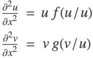
[3], Exact Solutions > Systems of Ordinary Differential Equations > Nonlinear Systems of Two Ordinary Differential Equations, 3.2.7
ClearAll[f, g]
rls = {f -> Sin, g -> Cos};
op = {Inactive[Plus][Inactive[Div][Inactive[Grad][u[x], {x}], {x}], -u[x] * f[v[x] / u[x]] ],
	Inactive[Plus][Inactive[Div][Inactive[Grad][v[x], {x}], {x}], -v[x] * g[v[x] / u[x]] ]
	} /. rls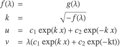
ClearAll[k]
params = Flatten[{FindRoot[f[λ] == g[λ] /. rls//Evaluate, {λ, 1 / 2}],
k -> Sqrt[f[λ]] /. rls, C[1] -> 1, C[2] -> 2}];
ares = Function[x, Evaluate[(C[1] * Exp[k * x] + C[2] * Exp[-k * x]) //. params]]
bres = Function[x, Evaluate[(λ * (C[1] * Exp[k * x] + C[2] * Exp[-k * x]) //. params)]]No boundary conditions are specified; they are deduced from the analytical solution.
bcs = {{DirichletCondition[u[x] == ares[0], x == 0], DirichletCondition[u[x] == ares[1], x == 1]}, {DirichletCondition[v[x] == bres[0], x == 0], DirichletCondition[v[x] == bres[1], x == 1]}} //. paramsregion = Line[{{0}, {1}}]Test 1:
VerificationTest[
	{nlfun1, nlfun2} = NDSolveValue[{op == {0, 0}, bcs}, {u, v}, Element[{x}, region], Method -> sopts, InitialSeeding -> {u[x] == 1, v[x] == x}];
	{Norm[Table[nlfun1[x] - ares[x], {x, 0, 1, 0.1}]] < 10 ^ -8, Norm[Table[nlfun2[x] - bres[x], {x, 0, 1, 0.1}]] < 10 ^ -8},
	{True, True},
	TestID -> "FEM-NL-Stationary-1D-System-Reaction-0001-A"
	]
Test 2:
VerificationTest[
	{anlfun1, anlfun2} = NDSolveValue[{Activate[op == {0, 0}], bcs}, {u, v}, Element[{x}, region], Method -> sopts, InitialSeeding -> {u[x] == 1, v[x] == x}];
	{Norm[Table[anlfun1[x] - ares[x], {x, 0, 1, 0.1}]] < 10 ^ -8, Norm[Table[anlfun2[x] - bres[x], {x, 0, 1, 0.1}]] < 10 ^ -8}
	,
	{True, True},
	TestID -> "FEM-NL-Stationary-1D-System-Reaction-0001-B"
	]
Test 3 & 4:
vd = NDSolve`VariableData[{"Dependent", "Space"} -> {{u, v}, {x}}];
nr = ToNumericalRegion[region];
sd = NDSolve`SolutionData[{"Dependent", "Space"} -> {{1, x}, nr}];
md = InitializePDEMethodData[vd, sd];
ibcs = InitializeBoundaryConditions[vd, sd, bcs];VerificationTest[
pdec = InitializePDECoefficients[vd, sd
, "DiffusionCoefficients" -> {{{{1}}, {{0}}}, {{{0}}, {{1}}}}
, "ReactionCoefficients" -> {{-Sin[v[x] / u[x]], 0}, {0, -Cos[v[x] / u[x]]}}
];
j = e = s = 0;
sdNew = PDESolve[pdec, ibcs, vd, sd, md,
"FindRootOptions" -> {Jacobian -> {Automatic, EvaluationMonitor :> j++}, EvaluationMonitor :> e++, StepMonitor :> s++}
];
{eif1, eif2} = ProcessPDESolutions[md, sdNew];
{Norm[Table[eif1[x] - ares[x], {x, 0, 1, 0.1}]] < 10 ^ -8, Norm[Table[eif2[x] - bres[x], {x, 0, 1, 0.1}]] < 10 ^ -8, e == 7, s == 6, j == 1}
,
{True, True, True, True, True},
{TestID -> "FEM-NL-Stationary-1D-System-Reaction-0001-C"}
]VerificationTest[
pdec = InitializePDECoefficients[vd, sd
, "DiffusionCoefficients" -> {{{{1}}, {{0}}}, {{{0}}, {{1}}}}
, "LoadCoefficients" -> {{Sin[v[x] / u[x]] * u[x]}, {Cos[v[x] / u[x]] * v[x]}}
];
j = e = s = 0;
sdNew = PDESolve[pdec, ibcs, vd, sd, md,
"FindRootOptions" -> {Jacobian -> {Automatic, EvaluationMonitor :> j++}, EvaluationMonitor :> e++, StepMonitor :> s++}
];
{eif1, eif2} = ProcessPDESolutions[md, sdNew];
{Norm[Table[eif1[x] - ares[x], {x, 0, 1, 0.1}]] < 10 ^ -8, Norm[Table[eif2[x] - bres[x], {x, 0, 1, 0.1}]] < 10 ^ -8, e == 7, s == 6, j == 1}
,
{True, True, True, True, True},
{TestID -> "FEM-NL-Stationary-1D-System-Reaction-0001-D"}
]2D Single Equation
This section contains examples of nonlinear partial differential equations with one equation.
Diffusion—FEM-NL-Stationary-2D-Single-Diffusion-0001
Test Reference:
[3], Exact Solutions > Nonlinear Partial Differential Equations > Other Second-Order Partial Differential Equations; Equation 4.1.2; Equation of steady transonic gas flow.
op = Inactive[Plus][Inactive[Div][{{b D[u[x, y], x], 0}, {0, 1}}. Inactive[Grad][u[x, y], {x, y}], {x, y}], a / y D[u[x, y], y]]params = {C[1] -> 1, C[2] -> 1, C[3] -> 1, C[4] -> 1, a -> 1, b -> 1};
ares = Function[{x, y}, Evaluate[-(b C[1]) / (2(a + 1)) y ^ 2 + C[2]y ^ (1 - a) + C[3] + 2 / (3 C[1])(C[1]x + C[4]) ^ (3 / 2) /. params]]Activate[op /. u -> ares /. params]No boundary conditions are specified; they are deduced from the analytical solution.
bcs = {DirichletCondition[u[x, y] == ares[x, y], True]}region = Rectangle[{1, 1}, {2, 3}]Tests 1:
VerificationTest[
	nlfun = NDSolveValue[{op == 0, bcs} /. params, u, Element[{x, y}, region], Method -> sopts, InitialSeeding -> {u[x, y] == 2 + Sqrt[2] / 3 + Sqrt[2] * x - y ^ 2 / 4}];
	Norm[Table[nlfun[x, y] - ares[x, y], {x, 1, 2, 0.1}, {y, 1, 3, 0.1}]] < 10 ^ -4,
	True,
	TestID -> "FEM-NL-Stationary-2D-Single-Diffusion-0001-A"
	]
Tests 2:
In the activated case, the linearization leads to a higher-than-first-order derivative in the PDE coefficients, which can not be handled.
VerificationTest[
	anlfun = NDSolveValue[{Activate[op] == 0, bcs} /. params, u, Element[{x, y}, region], Method -> sopts, InitialSeeding -> {u[x, y] == 2 + Sqrt[2] / 3 + Sqrt[2] * x - y ^ 2 / 4}];
	Head[anlfun] === NDSolveValue,
	True,
	NDSolveValue::femnlmdor,
	TestID -> "FEM-NL-Stationary-2D-Single-Diffusion-0001-B"
	]
Test 3:
vd = NDSolve`VariableData[{"Dependent", "Space"} -> {{u}, {x, y}}];
nr = ToNumericalRegion[region];
sd = NDSolve`SolutionData[{"Dependent", "Space"} -> {{2 + Sqrt[2] / 3 + Sqrt[2] * x - y ^ 2 / 4}, nr}];
md = InitializePDEMethodData[vd, sd];
ibcs = InitializeBoundaryConditions[vd, sd, {bcs}];VerificationTest[
pdec = InitializePDECoefficients[vd, sd
, "DiffusionCoefficients" -> {{{{b D[u[x, y], x], 0}, {0, 1}}}} /. params
, "ConvectionCoefficients" -> {{{{0, a / y}}}} /. params
];
j = e = s = 0;
sdNew = PDESolve[pdec, ibcs, vd, sd, md,
"FindRootOptions" -> {Jacobian -> {Automatic, EvaluationMonitor :> j++}, EvaluationMonitor :> e++, StepMonitor :> s++}
];
{eif} = ProcessPDESolutions[md, sdNew];{Norm[Table[eif[x, y] - ares[x, y], {x, 1, 2, 0.1}, {y, 1, 3, 0.1}]] < 10 ^ -4, e == 16, s == 14, j == 2}
,
{True, True, True, True},
{TestID -> "FEM-NL-Stationary-2D-Single-Diffusion-0001-C"}
]Reaction—FEM-NL-Stationary-2D-Single-Reaction-0001
Test Reference:
[3], Exact Solutions > Nonlinear Partial Differential Equations > Second-Order Elliptic Partial Differential Equations; Equation 3.1.2;
rls = {a -> -1, b -> 2, n -> 2};
op = Inactive[Plus][Inactive[Div][-{{1, 0}, {0, 1}}. Inactive[Grad][u[x, y], {x, y}], {x, y}], a u[x, y] ^ n, b u[x, y] ^ (2 * n - 1)] /. rlsrls2 = {C[1] -> π / 4, C[2] -> -1};
ares = Function[{x, y}, Evaluate[((a * (1 - n) ^ 2 / (2 * (n + 1))) * (x * Sin[C[1]] + y * Cos[C[1]] + C[2]) ^ 2 - (b * (n + 1)) / (2 * a * n)) ^ (1 / (1 - n)) /. Flatten[{rls, rls2}]]]No boundary conditions are specified; they are deduced from the analytical solution.
bcs = {DirichletCondition[u[x, y] == ares[x, y], True]}region = Rectangle[{-1, -1}, {1, 1}]Tests 1:
VerificationTest[
	nlfun = NDSolveValue[{op == 0, bcs}, u, Element[{x, y}, region], Method -> sopts];
	Norm[Table[nlfun[x, y] - ares[x, y], {x, -1, 1, 0.1}, {y, -1, 1, 0.1}]] < 10 ^ -4,
	True,
	TestID -> "FEM-NL-Stationary-2D-Single-Reaction-0001-A"
	]
Tests 2:
VerificationTest[
	anlfun = NDSolveValue[{Activate[op == 0], bcs}, u, Element[{x, y}, region], Method -> sopts];
	Norm[Table[anlfun[x, y] - ares[x, y], {x, -1, 1, 0.1}, {y, -1, 1, 0.1}]] < 10 ^ -4,
	True,
	TestID -> "FEM-NL-Stationary-2D-Single-Reaction-0001-B"
	]
Tests 3 & 4:
vd = NDSolve`VariableData[{"Dependent", "Space"} -> {{u}, {x, y}}];
nr = ToNumericalRegion[region];
sd = NDSolve`SolutionData[{"Dependent", "Space"} -> {{1}, nr}];
md = InitializePDEMethodData[vd, sd];
ibcs = InitializeBoundaryConditions[vd, sd, {bcs}];VerificationTest[
pdec = InitializePDECoefficients[vd, sd
, "DiffusionCoefficients" -> {{{{-1, 0}, {0, -1}}}}
, "ReactionCoefficients" -> {{(a u[x, y] ^ n + b u[x, y] ^ (2 * n - 1)) / u[x, y]}} /. rls
];
j = e = s = 0;
sdNew = PDESolve[pdec, ibcs, vd, sd, md,
"FindRootOptions" -> {Jacobian -> {Automatic, EvaluationMonitor :> j++}, EvaluationMonitor :> e++, StepMonitor :> s++}
];
{eif} = ProcessPDESolutions[md, sdNew];{Norm[Table[eif[x, y] - ares[x, y], {x, -1, 1, 0.1}, {y, -1, 1, 0.1}]] < 10 ^ -4, e == 10, s == 9, j == 1}
,
{True, True, True, True},
{TestID -> "FEM-NL-Stationary-2D-Single-Reaction-0001-C"}
]VerificationTest[
pdec = InitializePDECoefficients[vd, sd
, "DiffusionCoefficients" -> {{{{-1, 0}, {0, -1}}}}
, "LoadCoefficients" -> {-{a u[x, y] ^ n + b u[x, y] ^ (2 * n - 1)}} /. rls
];
j = e = s = 0;
sdNew = PDESolve[pdec, ibcs, vd, sd, md,
"FindRootOptions" -> {Jacobian -> {Automatic, EvaluationMonitor :> j++}, EvaluationMonitor :> e++, StepMonitor :> s++}
];
{eif} = ProcessPDESolutions[md, sdNew];{Norm[Table[eif[x, y] - ares[x, y], {x, -1, 1, 0.1}, {y, -1, 1, 0.1}]] < 10 ^ -4, e == 10, s == 9, j == 1}
,
{True, True, True, True},
{TestID -> "FEM-NL-Stationary-2D-Single-Reaction-0001-D"}
]Transient Tests
This section contains examples of time-dependent nonlinear partial differential equations used for testing.
1D Single Equation
This section contains examples of time dependent ordinary nonlinear differential equations with one equation. Ordinary differential equations with one independent variable are a special case of partial differential equations that usually deal with more than one independent variable.
Diffusion—FEM-NL-Transient-1D-Single-Diffusion-0001
Test Reference:
[3], Exact Solutions > Nonlinear Partial Differential Equations >Second-Order Parabolic Partial Differential Equations > Heat Equation with a Power-Law Nonlinearity; Equation 1.2.1; Heat equation with a power-law nonlinearity.
op = D[u[t, x], t] + a Inactive[Div][{{-u[t, x]^m}}. Inactive[Grad][u[t, x], {x}], {x}]params = {a -> 2, λ -> 3, m -> 3}ares = Function[{t, x}, Evaluate[(λ m / a x + λ m / a λ t + 1) ^ (1 / m) /. params]]No boundary conditions are specified; they are deduced from the analytical solution.
bcs = {DirichletCondition[u[t, x] == ares[t, x], True]}No initial conditions are specified; they are deduced from the analytical solution.
ics = {u[0, x] == ares[0, x]}region = Line[{{0}, {1}}]Test 1:
VerificationTest[
	nlfun = NDSolveValue[{op == 0, bcs, ics} /. params, u, {t, 0, 1}, Element[{x}, region], Method -> topts];
	Norm[Table[nlfun[t, x] - ares[t, x] /. params, {t, 0, 1, 0.1}, {x, 0, 1, 0.1}]] < 10 ^ -2,
	True,
	TestID -> "FEM-NL-Transient-1D-Single-Diffusion-0001-A"
	]
Test 2:
VerificationTest[
	aeqn = Activate[{op == 0, bcs, ics} /. params];
	anlfun = NDSolveValue[aeqn, u, {t, 0, 1}, Element[{x}, region], Method -> topts];
	Norm[Table[anlfun[t, x] - ares[t, x], {t, 0, 1, 0.1}, {x, 0, 1, 0.1}]] < 10 ^ -2,
	True,
	TestID -> "FEM-NL-Transient-1D-Single-Diffusion-0001-B"
]Diffusion—FEM-NL-Transient-1D-Single-Diffusion-0002
Test Reference:
[3], Exact Solutions > Nonlinear Partial Differential Equations >Second-Order Parabolic Partial Differential Equations > Heat Equation with a Exponential Nonlinearity; Equation 1.2.7; Heat Equation with a Exponential Nonlinearity.
op = D[u[t, x], t] + a Inactive[Div][{{-Exp[λ u[t, x]]}}. Inactive[Grad][u[t, x], {x}], {x}]params = {A -> 1, B -> 2, λ -> 3, a -> 1 / 2}ares = Function[{t, x}, Evaluate[2 / λ Log[(x + A) / Sqrt[B - 2 a t]] /. params]]No boundary conditions are specified; they are deduced from the analytical solution.
bcs = {DirichletCondition[u[t, x] == ares[t, x], True]}No initial conditions are specified; they are deduced from the analytical solution.
ics = {u[0, x] == ares[0, x]}region = Line[{{0}, {1}}]Test 1:
VerificationTest[
	nlfun = NDSolveValue[{op == 0, bcs, ics} /. params, u, {t, 0, 1}, Element[{x}, region], Method -> topts];
	Norm[Table[nlfun[t, x] - ares[t, x], {t, 0, 1, 0.1}, {x, 0, 1, 0.1}]] < 10 ^ -2,
	True,
	TestID -> "FEM-NL-Transient-1D-Single-Diffusion-0002-A"
	]
Test 2:
VerificationTest[
	aeqn = Activate[{op == 0, bcs, ics} /. params];
	anlfun = NDSolveValue[aeqn, u, {t, 0, 1}, Element[{x}, region], Method -> topts];
	Norm[Table[anlfun[t, x] - ares[t, x], {t, 0, 1, 0.1}, {x, 0, 1, 0.1}]] < 10 ^ -2,
	True,
	TestID -> "FEM-NL-Transient-1D-Single-Diffusion-0002-B"
]Diffusion—FEM-NL-Transient-1D-Single-Diffusion-0003
Test Reference:
[3], Exact Solutions > Nonlinear Partial Differential Equations > Second-Order Hyperbolic Partial Differential Equations; Equation 2.2.1;
op = D[u[t, x], {t, 2}] + a Inactive[Div][{{-u[t, x]}}. Inactive[Grad][u[t, x], {x}], {x}]params = {A -> 2, B -> 3, C -> -1, a -> 2}ares = Function[{t, x}, Evaluate[1 / 2a A ^ 2 t ^ 2 + B t + A x + C /. params]]No boundary conditions are specified; they are deduced from the analytical solution.
bcs = {DirichletCondition[u[t, x] == ares[t, x], True]}No initial conditions are specified; they are deduced from the analytical solution.
ics = {u[0, x] == ares[0, x], Derivative[1, 0][u][0, x] == D[ares[t, x], t] /. t -> 0}region = Line[{{0}, {1}}]Test 1:
VerificationTest[
	nlfun = NDSolveValue[{op == 0, bcs, ics} /. params, u, {t, 0, 1}, Element[{x}, region], Method -> topts];
	Norm[Table[nlfun[t, x] - ares[t, x], {t, 0, 1, 0.1}, {x, 0, 1, 0.1}]] < 10 ^ -3,
	True,
	TestID -> "FEM-NL-Transient-1D-Single-Diffusion-0003-A"
]Convection—FEM-NL-Transient-1D-Single-Convection-0001
Test Reference:
[3], Exact Solutions > Nonlinear Partial Differential Equations >Second-Order Parabolic Partial Differential Equations > Burgers Equation; Equation 1.3.1; Burgers equation.
op = D[u[t, x], t] + Inactive[Plus][Inactive[Div][{{-1}}. Inactive[Grad][u[t, x], {x}], {x}], -u[t, x] * D[u[t, x], x]]params = {C[1] -> 1, λ -> 1}ares = Function[{t, x}, Evaluate[λ + 2 / (x + λ t + C[1]) /. params]]No boundary conditions are specified; they are deduced from the analytical solution.
bcs = {DirichletCondition[u[t, x] == ares[t, x], True]}No initial conditions are specified; they are deduced from the analytical solution.
ics = {u[0, x] == ares[0, x]}region = Line[{{0}, {1}}]Test 1:
VerificationTest[
	nlfun = NDSolveValue[{op == 0, bcs, ics} /. params, u, {t, 0, 1}, Element[{x}, region], Method -> topts];
	Norm[Table[nlfun[t, x] - ares[t, x], {t, 0, 1, 0.1}, {x, 0, 1, 0.1}]] < 10 ^ -2,
	True,
	TestID -> "FEM-NL-Transient-1D-Single-Convection-0001-A"
	]
Test 2:
VerificationTest[
	aeqn = Activate[{op == 0, bcs, ics} /. params];
	anlfun = NDSolveValue[aeqn, u, {t, 0, 1}, Element[{x}, region], Method -> topts];
	Norm[Table[anlfun[t, x] - ares[t, x], {t, 0, 1, 0.1}, {x, 0, 1, 0.1}]] < 10 ^ -2,
	True,
	TestID -> "FEM-NL-Transient-1D-Single-Convection-0001-B"
]Convection—FEM-NL-Transient-1D-Single-Convection-0002
Test Reference:
https://mathematica.stackexchange.com/q/10453/18437
op = D[u[t, x], t] + Inactive[Plus][Inactive[Div][{{-c}}. Inactive[Grad][u[t, x], {x}], {x}], +u[t, x] * D[u[t, x], x]]params = {β -> 4, c -> 1 / 20, α -> 5}ares = Function[{t, x}, Evaluate[(2 π β c Exp[-c π ^ 2t]Sin[π x]) / (α + β Exp[-c π ^ 2t]Cos[π x]) /. params]]Boundary conditions are deduced from the analytical solution.
bcs = {DirichletCondition[u[t, x] == 0, True]}Initial conditions are deduced from the analytical solution.
ics = {u[0, x] == ares[0, x]}region = Line[{{0}, {1}}]Test 1:
VerificationTest[
	nlfun = NDSolveValue[{op == 0, bcs, ics} /. params, u, {t, 0, 2}, Element[{x}, region], Method -> topts];
	Norm[Table[nlfun[t, x] - ares[t, x], {t, 0, 1, 0.1}, {x, 0, 1, 0.1}]] < 10 ^ -3,
	True,
	TestID -> "FEM-NL-Transient-1D-Single-Convection-0002-A"
	]
Test 2:
VerificationTest[
	aeqn = Activate[{op == 0, bcs, ics} /. params];
	anlfun = NDSolveValue[aeqn, u, {t, 0, 1}, Element[{x}, region], Method -> topts];
	Norm[Table[anlfun[t, x] - ares[t, x], {t, 0, 1, 0.1}, {x, 0, 1, 0.1}]] < 10 ^ -3,
	True,
	TestID -> "FEM-NL-Transient-1D-Single-Convection-0002-B"
]Reaction—FEM-NL-Transient-1D-Single-Reaction-0001
Test Reference:
[3], Exact Solutions > Nonlinear Partial Differential Equations >Second-Order Parabolic Partial Differential Equations > Fisher Equation; Equation 1.1.1; Fisher equation.
op = D[u[t, x], t] + Inactive[Plus][Inactive[Div][{{-1}}. Inactive[Grad][u[t, x], {x}], {x}], -a * u[t, x] * (1 - u[t, x])]params = {C -> 1, a -> 2 / 3}ares = Function[{t, x}, Evaluate[1 / (1 + C Exp[-5 / 6 a t - 1 / 6 Sqrt[6 a]x]) ^ 2 /. params]]No boundary conditions are specified; they are deduced from the analytical solution.
bcs = {DirichletCondition[u[t, x] == ares[t, 0], x == 0], DirichletCondition[u[t, x] == ares[t, 1], x == 1]}No initial conditions are specified; they are deduced from the analytical solution.
ics = {u[0, x] == ares[0, x]}region = Line[{{0}, {1}}]Test 1:
VerificationTest[
	nlfun = NDSolveValue[{op == 0, bcs, ics} /. params, u, {t, 0, 1}, Element[{x}, region], Method -> topts];
	Norm[Table[nlfun[t, x] - ares[t, x], {t, 0, 1, 0.1}, {x, 0, 1, 0.1}]] < 10 ^ -3,
	True,
	TestID -> "FEM-NL-Transient-1D-Single-Reaction-0001-A"
	]
Test 2:
VerificationTest[
	aeqn = Activate[{op == 0, bcs, ics} /. params];
	anlfun = NDSolveValue[aeqn, u, {t, 0, 1}, Element[{x}, region], Method -> topts];
	Norm[Table[anlfun[t, x] - ares[t, x], {t, 0, 1, 0.1}, {x, 0, 1, 0.1}]] < 10 ^ -3,
	True,
	TestID -> "FEM-NL-Transient-1D-Single-Reaction-0001-B"
]Reaction—FEM-NL-Transient-1D-Single-Reaction-0002
Test Reference:
[3], Exact Solutions > Nonlinear Partial Differential Equations >Second-Order Hyperbolic Partial Differential Equations > Klein–Gordon Equation with a Power-Law Nonlinearity; Equation 2.1.1; Klein--Gordon equation with a power-law nonlinearity.
op = D[u[t, x], {t, 2}] + Inactive[Plus][Inactive[Div][{{-1}}. Inactive[Grad][u[t, x], {x}], {x}], -a * u[t, x] - b u[t, x] ^ n]params = {C[1] -> -1, C[2] -> -1, a -> 1, b -> 1, n -> 2}a > 0 && b (n + 1) > 0 /. paramsares = Function[{t, x}, Evaluate[Block[{z = 1 / 2 Sqrt[a](1 - n)(x Sinh[C[1]] + t Cosh[C[1]]) + C[2]}, ((2 b Sinh[z] ^ 2) / (a * (n + 1))) ^ (1 / (1 - n))] /. params]]No boundary conditions are specified; they are deduced from the analytical solution.
bcs = {DirichletCondition[u[t, x] == ares[t, 0], x == 0], DirichletCondition[u[t, x] == ares[t, 1], x == 1]}No initial conditions are specified; they are deduced from the analytical solution.
ics = {u[0, x] == ares[0, x], Derivative[1, 0][u][0, x] == D[ares[t, x], t] /. t -> 0}region = Line[{{0}, {1}}]Test 1:
VerificationTest[
	nlfun = NDSolveValue[{op == 0, bcs, ics} /. params, u, {t, 0, 1}, Element[{x}, region], Method -> topts];
	Norm[Table[nlfun[t, x] - ares[t, x], {t, 0, 1, 0.1}, {x, 0, 1, 0.1}]] < 10 ^ -2,
	True,
	TestID -> "FEM-NL-Transient-1D-Single-Reaction-0002-A"
	]
Test 2:
VerificationTest[
	aeqn = Activate[{op == 0, bcs, ics} /. params];
	anlfun = NDSolveValue[aeqn, u, {t, 0, 1}, Element[{x}, region], Method -> topts];
	Norm[Table[anlfun[t, x] - ares[t, x], {t, 0, 1, 0.1}, {x, 0, 1, 0.1}]] < 10 ^ -2,
	True,
	TestID -> "FEM-NL-Transient-1D-Single-Reaction-0002-B"
]Load—FEM-NL-Transient-1D-Single-Load-0001
Test Reference:
[3], Exact Solutions > Nonlinear Partial Differential Equations >Second-Order Parabolic Partial Differential Equations > Equation 1.1.5;
op = D[u[t, x], t] + Inactive[Plus][Inactive[Div][{{-1}}. Inactive[Grad][u[t, x], {x}], {x}], -a, -b Exp[λ u[t, x]]]params = {C -> -1, a -> 1, b -> -2, λ -> 3 / 2}ares = Function[{t, x}, Evaluate[-2 / λ Log[Sqrt[-b / a] + C Exp[-Sqrt[a λ / 2]x - 1 / 2a λ t]] /. params]]No boundary conditions are specified; they are deduced from the analytical solution.
bcs = {DirichletCondition[u[t, x] == ares[t, 0], x == 0], DirichletCondition[u[t, x] == ares[t, 1], x == 1]}No initial conditions are specified; they are deduced from the analytical solution.
ics = {u[0, x] == ares[0, x]}region = Line[{{0}, {1}}]Test 1:
VerificationTest[
	nlfun = NDSolveValue[{op == 0, bcs, ics} /. params, u, {t, 0, 1}, Element[{x}, region], Method -> topts];
	Norm[Table[nlfun[t, x] - ares[t, x], {t, 0, 1, 0.1}, {x, 0, 1, 0.1}]] < 10 ^ -3,
	True,
	TestID -> "FEM-NL-Transient-1D-Single-Load-0001-A"
	]
Test 2:
VerificationTest[
	aeqn = Activate[{op == 0, bcs, ics} /. params];
	anlfun = NDSolveValue[aeqn, u, {t, 0, 1}, Element[{x}, region], Method -> topts];
	Norm[Table[anlfun[t, x] - ares[t, x], {t, 0, 1}, {x, 0, 1, 0.1}]] < 10 ^ -3,
	True,
	TestID -> "FEM-NL-Transient-1D-Single-Load-0001-B"
]Load—FEM-NL-Transient-1D-Single-Load-0002
Test Reference:
[3], Exact Solutions > Nonlinear Partial Differential Equations >Second-Order Hyperbolic Partial Differential Equations > Modified Liouville Equation; Equation 2.1.3;
op = D[u[t, x], {t, 2}] + Inactive[Plus][a ^ 2 Inactive[Div][{{-1}}. Inactive[Grad][u[t, x], {x}], {x}], -b Exp[β u[t, x]]]params = {A -> 1, B -> 2, C -> 1, a -> 1, b -> 1, β -> 3 / 2}ares = Function[{t, x}, Evaluate[1 / β Log[2(B ^ 2 - a ^ 2A ^ 2) / (b β (A x + B t + C) ^ 2)] /. params]]No boundary conditions are specified; they are deduced from the analytical solution.
bcs = {DirichletCondition[u[t, x] == ares[t, 0], x == 0], DirichletCondition[u[t, x] == ares[t, 1], x == 1]}No initial conditions are specified; they are deduced from the analytical solution.
ics = {u[0, x] == ares[0, x], Derivative[1, 0][u][0, x] == D[ares[t, x], t] /. t -> 0}region = Line[{{0}, {1}}]Test 1:
VerificationTest[
	nlfun = NDSolveValue[{op == 0, bcs, ics} /. params, u, {t, 0, 1}, Element[{x}, region], Method -> topts];
	Norm[Table[nlfun[t, x] - ares[t, x], {t, 0, 1, 0.1}, {x, 0, 1, 0.1}]] < 10 ^ -2,
	True,
	TestID -> "FEM-NL-Transient-1D-Single-Load-0002-A"
	]
Test 2:
VerificationTest[
	aeqn = Activate[{op == 0, bcs, ics} /. params];
	anlfun = NDSolveValue[aeqn, u, {t, 0, 1}, Element[{x}, region], Method -> topts];
	Norm[Table[anlfun[t, x] - ares[t, x], {t, 0, 1, 0.1}, {x, 0, 1, 0.1}]] < 10 ^ -2,
	True,
	TestID -> "FEM-NL-Transient-1D-Single-Load-0002-B"
	]
Test 3:
VerificationTest[
	nlfun = NDSolveValue[{op == 0, bcs, ics} /. params, u, {t, 0, 1}, Element[{x}, region], Method -> topts, "MaxStepSize" -> Max[Abs[Subtract@@@Partition[anlfun["Coordinates"][[1]], 2, 1]]]];
	Norm[Table[nlfun[t, x] - ares[t, x], {t, 0, 1, 0.1}, {x, 0, 1, 0.1}]] < 10 ^ -2,
	True,
	TestID -> "FEM-NL-Transient-1D-Single-Load-0002-C"
]VerificationTest[
nlfun = NDSolveValue[{D[u[t, x], {t, 2}] + Plus[a ^ 2 Inactive[Div][{{-1}}. Inactive[Grad][u[t, x], {x}], {x}], -b Exp[β u[t, x]]] == 0, bcs, ics} /. params, u, {t, 0, 1}, Element[{x}, region], Method -> topts];
Norm[Table[nlfun[t, x] - ares[t, x], {t, 0, 1, 0.1}, {x, 0, 1, 0.1}]] < 10 ^ -2,
True,
TestID -> "FEM-NL-Transient-1D-Single-Load-0002-D"
]Reaction-Diffusion—FEM-NL-Transient-1D-Single-Reaction-Diffusion-0001
Test Reference:
[3], Exact Solutions > Nonlinear Partial Differential Equations >Second-Order Parabolic Partial Differential Equations > Fisher Equation; Equation 1.2.5;
op = D[u[t, x], t] + Inactive[Plus][a Inactive[Div][{{-u[t, x] ^ (2 n)}}. Inactive[Grad][u[t, x], {x}], {x}], -b * u[t, x] ^ (1 - n)]params = {C[1] -> 0, C[2] -> 5, a -> 1, b -> 0, n -> 1}ares = Function[{t, x}, Evaluate[With[{k = 2a(n + 1) / n}, ((x + C[1]) / Sqrt[C[2] - k t] - (b n ^ 2) / (3 a (n + 1))(C[2] - k t)) ^ (1 / n)] /. params]]No boundary conditions are specified; they are deduced from the analytical solution.
bcs = {DirichletCondition[u[t, x] == ares[t, x], True]}No initial conditions are specified; they are deduced from the analytical solution.
ics = {u[0, x] == ares[0, x]}region = Line[{{1}, {2}}]Test 1:
VerificationTest[
	nlfun = NDSolveValue[{op == 0, bcs, ics} /. params, u, {t, 0, 1}, Element[{x}, region], Method -> topts];
	Norm[Table[nlfun[t, x] - ares[t, x], {t, 0, 0.1, 0.01}, {x, 1, 2, 0.1}]] < 10 ^ -3,
	True,
	TestID -> "FEM-NL-Transient-1D-Single-Reaction-Diffusion-0001-A"
	]
Test 2:
VerificationTest[
	aeqn = Activate[{op == 0, bcs, ics} /. params];
	anlfun = NDSolveValue[Activate[{op == 0, bcs, ics}] /. params, u, {t, 0, 1}, Element[{x}, region], Method -> topts];
	Norm[Table[anlfun[t, x] - ares[t, x], {t, 0, 0.1, 0.01}, {x, 1, 2, 0.1}]] < 10 ^ -3,
	True,
	TestID -> "FEM-NL-Transient-1D-Single-Reaction-Diffusion-0001-B"
	]
2D Single Equation
This section contains examples of time-dependent partial nonlinear differential equations with one equation.
Diffusion—FEM-NL-Stationary-2D-Single-Diffusion-0001
Test Reference:
[5], Example 6.3.6, page 100
op = 175 D[u[t, x, y], t] + Inactive[Div][-{{k[u[t, x, y]], 0}, {0, k[u[t, x, y]]}}. Inactive[Grad][u[t, x, y], {x, y}], {x, y}] /. k :> Function[u, 1 / 200 u + 1];ares = Function[{t, x, y}, 68(1 + Cos[π x / 2])(1 + Cos[π y / 2])Exp[-t]]f = Activate[op /. u -> ares]bcs = {DirichletCondition[u[t, x, y] == 0, True]}No initial conditions are specified; they are deduced from the analytical solution.
ics = {u[0, x, y] == ares[0, x, y]}region = Rectangle[{-2, -2}, {2, 2}]Tests 1:
VerificationTest[
	nlfun = NDSolveValue[{op == f, bcs, ics}, u, {t, 0, 1}, Element[{x, y}, region], MaxStepSize -> 0.01];
	Norm[Table[nlfun[1, x, y] - ares[1, x, y], {x, -2, 2, 0.1}, {y, -2, 2, 0.1}]] < 10 ^ -1,
	True,
	TestID -> "FEM-NL-Transient-2D-Single-Diffusion-0001-A"
	]
A higher-quality result can be achieved by reducing the max cell measure of the mesh and further reducing the max step size. This is not done here because the test will run longer.
Test Result Inspection
This section contains the evaluation of the test runs. It works by collecting all instances of TestResultObject and generating a TestReport.
nb = EvaluationNotebook[];
cso = Cells[nb, CellStyle -> {"Output"}];
tros = Cases[ToExpression[First[NotebookRead[#]]]& /@ cso, _TestResultObject];
report = TestReport[tros]Column /@ (Normal /@ report["TestsFailed"])//TabViewIf the preceding table is empty, all tests succeeded.
References
[1] Advanced Topics in Finite Element Analysis of Structures; Bhatti, M. Asghar; Wiley; ISBN: 978-81-265-4537-7.
[2] Nonlinear Finite Element Analysis; Reddy, J. N.; Oxford; ISBN: 978-0-19-852529-5.
[3] "EqWorld, The World of Mathematical Equations"; http://eqworld.ipmnet.ru.
[4] Automated Solution of Differential Equations by the Finite Element Method; Logg, A; Mardal, K-A; Wells, G. N.; Springer; ISBN: 978-3-642-23098-1.
[5] "Nonlinear, Transient Conduction Heat Transfer Using a Discontinuous Galerkin Hierarchical Finite Element Method"; Sanders, J. C.; http://www.phys.uconn.edu/~sanders/ThesisMain.pdf.