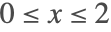
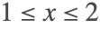
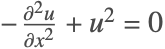
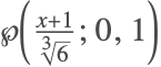
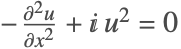
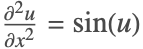
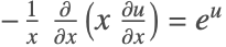
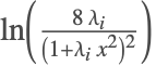
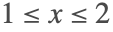
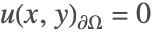
非線形有限法の検証テスト

定常テスト	テスト結果の調査
非定常テスト	参考文献

このノートブックには，非線形の有限要素法が予期する通りに作動するかどうかを検証するテストが含まれている．すべてのテストを実行する場合には，SelectAllを使い，Shift+Enterを押す．すると結果が「テスト結果の調査」のセクションに表示される．

テスト中の微分方程式は通常非アクティブな形式で与えられる．場合によっては，微分方程式の非アクティブ形式のみで特定の微分方程式を設定できるということもある．実際にどのような場合に非アクティブな方程式が使われるかについての詳細は，「有限要素法の使用上のヒント」のチュートリアルで説明される．「形式的な偏微分方程式」と「ノイマン値と形式的な偏微分方程式」 aについてのセクションは特に関連している．厳密にはほとんどのテストにおいて非アクティブな形式は必要ではないが，方程式のペアもテストできるように，非アクティブ形式も用意されている．

これらのテストは，独自の微分方程式モデルを開発する基礎ともなるものである．このため，テストは定常（時間に依存する）と非定常（時間に依存しない）のテストにグループ分けされている．次に方程式の数によってグループ分けされている．単一方程式あるいは結合方程式が考慮される．それらのカテゴリでは，一次元と二次元のテストがある．三次元のテストがないのは，有限要素コードの実装による理由からである．すべての次元におけるコードの基本は同じであり，三次元のテストを含むことによる利点はあまりないからである．

実際のテスト内のセルの中には評価できないものもある．これらのセルには主に記号的な微分が含まれ，実行に余分なランタイムとメモリが必要である．本当の解析解が存在する場合には，関数として返される．微分をそこで調査することができる．これらのセルを評価可能にするためには，評価したいセルを選び，セル ▶ セルのプロパティを選んでから「評価可能」にチェックマークが入っていることを確かめる．

テストが意図されるように作動するためには，個々のサブテストも評価されなければならない．

最新の有限要素パッケージをロードする．

Wolfram Language code:

Needs["NDSolve`FEM`"]
Needs["MUnit`"]

有限要素法を使うようにオプションを設定する．

Wolfram Language code:

sopts = {"FiniteElement"};
topts = {"PDEDiscretization" -> {"MethodOfLines", "SpatialDiscretization" -> "FiniteElement"}};

多くのメモリを必要とする上の結果が保存されることを避けるために，履歴の長さを0に設定する．

Wolfram Language code: $HistoryLength = 0;

定常テスト

このセクションには，定常の（時間に依存しない）非線形偏微分方程式の例が含まれる．

一次元の単一方程式

このセクションには，方程式が1つである非線形の常微分方程式の例が含まれる．独立変数を1つ含む常微分方程式は，通常2つ以上の独立変数を扱う偏微分方程式の特別な場合である．

拡散—FEM-NL-Stationary-1D-Single-Diffusion-0001

テストの参考文献：

[1], chapter 7, page 341.

方程式：

非アクティブな形式で方程式を設定する．

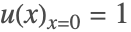
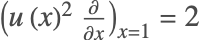
Wolfram Language code: op = Inactive[Div][{{-u[x] ^ 2}}. Inactive[Grad][u[x], {x}], {x}] - 4

解析解：

解析解を設定する．

Wolfram Language code: ares = Function[x, (-6x ^ 2 + 18x + 1) ^ (1 / 3)]

境界条件：

および

境界条件を設定する．

Wolfram Language code: bcs = {DirichletCondition[u[x] == 1., x == 0], NeumannValue[2., x == 1]}

領域：

領域を設定する．

Wolfram Language code: region = Line[{{0}, {1}}]

テスト1：

非アクティブな偏微分方程式をテストする．

Wolfram Language code:

VerificationTest[
	nlfun = NDSolveValue[{op == bcs[[2]], bcs[[1]]}, u, Element[{x}, region], Method -> sopts, InitialSeeding -> {u[x] == 1}];
	Norm[Table[nlfun[x] - ares[x], {x, 0, 1, 0.1}]] < 10 ^ -9, 
	True, 
	TestID -> "FEM-NL-Stationary-1D-Single-Diffusion-0001-A"
	]

テスト2：

アクティブな偏微分方程式をテストする．

Wolfram Language code:

VerificationTest[
	aeqn = Activate[op - bcs[[2]] == 0];
	anlfun = NDSolveValue[{aeqn, bcs[[1]]}, u, Element[{x}, region], Method -> sopts, InitialSeeding -> {u[x] == 1}];
	Norm[Table[anlfun[x] - ares[x], {x, 0, 1, 0.1}]] < 10 ^ -9, 
	True, 
	TestID -> "FEM-NL-Stationary-1D-Single-Diffusion-0001-B"
	]

テスト3：

ステップと評価の数をチェックしながら，低レベル関数をテストする．

Wolfram Language code:

VerificationTest[
	vd = NDSolve`VariableData[{"Dependent", "Space"} -> {{u}, {x}}];
	nr = ToNumericalRegion[region];
	sd = NDSolve`SolutionData[{"Dependent", "Space"} -> {{1}, nr}];
	md = InitializePDEMethodData[vd, sd];
	ibcs = InitializeBoundaryConditions[vd, sd, {bcs}];
	pdec = InitializePDECoefficients[vd, sd
	, "DiffusionCoefficients" -> {{{{-u[x] ^ 2}}}}
	, "LoadCoefficients" -> {{4}}
	];
	j = e = s = 0;
	sdNew = PDESolve[pdec, ibcs, vd, sd, md, 
	"FindRootOptions" -> {Jacobian -> {Automatic, EvaluationMonitor :> j++}, EvaluationMonitor :> e++, StepMonitor :> s++}
	];
	{eif} = ProcessPDESolutions[md, sdNew];
{Norm[Table[eif[x] - ares[x], {x, 0, 1, 0.1}]] < 10 ^ -9, e == 11, s == 10, j == 3}
	, 
	{True, True, True, True}, 
	{TestID -> "FEM-NL-Stationary-1D-Single-Diffusion-0001-C"}
	]

拡散—FEM-NL-Stationary-1D-Single-Diffusion-0002

テストの参考文献：

[4], page 38

方程式：

右辺 f は，解析解から計算される．

方程式を設定する．

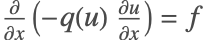
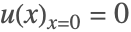
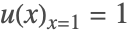
Wolfram Language code: op = Inactive[Div][{{-q[u[x]]}}. Inactive[Grad][u[x], {x}], {x}]

解析解：

解のパラメータを設定する．　　

Wolfram Language code: params = {q[u_] -> ((1 + u) ^ m), m -> 2}

解析解を設定する．

Wolfram Language code: ares = Function[{x}, Evaluate[((2 ^ (m + 1) - 1) * x + 1) ^ (1 / (m + 1)) - 1 //. params]]

右辺 f を設定する．

Wolfram Language code: f = Activate[op //. params] /. u -> ares

境界条件：

および

境界条件を設定する．

Wolfram Language code: bcs = {DirichletCondition[u[x] == 0., x == 0], DirichletCondition[u[x] == 1., x == 1]}

領域：

領域を設定する．

Wolfram Language code: region = Line[{{0}, {1}}]

テスト1：

非アクティブな形式の偏微分方程式をテストする．

Wolfram Language code:

VerificationTest[
	nlfun = NDSolveValue[{op == f, bcs} //. params, u, Element[{x}, region], Method -> sopts, InitialSeeding -> {u[x] == x}];
	Norm[Table[nlfun[x] - ares[x], {x, 0, 1, 0.1}]] < 10 ^ -8, 
	True, 
	TestID -> "FEM-NL-Stationary-1D-Single-Diffusion-0002-A"
	]

テスト2：

偏微分方程式をテストする．

Wolfram Language code:

VerificationTest[
	aeqn = Activate[op == f //. params];
	anlfun = NDSolveValue[{aeqn, bcs}, u, Element[{x}, region], Method -> sopts, InitialSeeding -> {u[x] == x}];
	Norm[Table[anlfun[x] - ares[x], {x, 0, 1, 0.1}]] < 10 ^ -8, 
	True, 
	TestID -> "FEM-NL-Stationary-1D-Single-Diffusion-0002-B"
	]

テスト3：

複数のメッシュブロックで低レベル関数をテストする．

Wolfram Language code:

VerificationTest[
	vd = NDSolve`VariableData[{"Dependent", "Space"} -> {{u}, {x}}];
	mesh = ToElementMesh[region, "MeshElementBlocks" -> 3];
	nr = ToNumericalRegion[mesh];
	sd = NDSolve`SolutionData[{"Dependent", "Space"} -> {{x}, nr}];
	md = InitializePDEMethodData[vd, sd];
	ibcs = InitializeBoundaryConditions[vd, sd, {bcs}];
	pdec = InitializePDECoefficients[vd, sd
	, "DiffusionCoefficients" -> {{{{-q[u[x]]}}}} //. params
	, "LoadCoefficients" -> {{f}}
	];
	sdNew = PDESolve[pdec, ibcs, vd, sd, md];
	{eif} = ProcessPDESolutions[md, sdNew];
	{Norm[Table[eif[x] - ares[x], {x, 0, 1, 0.1}]] < 10 ^ -8, Length[mesh["MeshElements"]]}
	, 
	{True, 3}, 
	{TestID -> "FEM-NL-Stationary-1D-Single-Diffusion-0002-C"}
	]

対流—FEM-NL-Stationary-1D-Single-Convection-0001

テストの参考文献：

[2], problems: 3.7, page 83.

方程式：

非アクティブな形式で方程式を設定する．

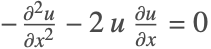
Wolfram Language code: op = Inactive[Div][{{-1}}. Inactive[Grad][u[x], {x}], {x}] - 2u[x] * D[u[x], x]

解析解：

解析解を設定する．

Wolfram Language code: ares = Function[x, 1 / (1 + x)]

境界条件：

および

境界条件を設定する．

Wolfram Language code: bcs = {DirichletCondition[u[x] == 1, x == 0], DirichletCondition[u[x] == 1 / 2, x == 1]}

領域：

領域を設定する．

Wolfram Language code: region = Line[{{0}, {1}}]

テスト1：

非アクティブな形式の偏微分方程式をテストする．

Wolfram Language code:

VerificationTest[
	nlfun = NDSolveValue[{op == 0, bcs}, u, Element[{x}, region], Method -> "FiniteElement", InitialSeeding -> {u[x] == 1}];
	Norm[Table[nlfun[x] - ares[x], {x, 0, 1, 0.1}]] < 10 ^ -7, 
	True, 
	TestID -> "FEM-NL-Stationary-1D-Single-Convection-0001-A"
	]

テスト2：

偏微分方程式をテストする．

Wolfram Language code:

VerificationTest[
	anlfun = NDSolveValue[{Activate[op == 0], bcs}, u, Element[{x}, region], Method -> "FiniteElement", InitialSeeding -> {u[x] == 1}];
	Norm[Table[anlfun[x] - ares[x], {x, 0, 1, 0.1}]] < 10 ^ -7, 
	True, 
	TestID -> "FEM-NL-Stationary-1D-Single-Convection-0001-B"
	]

テスト3：

低レベル関数をテストし，ステップと評価を管理する．

Wolfram Language code:

VerificationTest[
	nr = ToNumericalRegion[region];vd = NDSolve`VariableData[{"Dependent", "Space"} -> {{u}, {x}}];sd = NDSolve`SolutionData[{"Dependent", "Space"} -> {{1}, nr}];
	md = InitializePDEMethodData[vd, sd];ibcs = InitializeBoundaryConditions[vd, sd, {bcs}];
	pdec = InitializePDECoefficients[vd, sd
	, "DiffusionCoefficients" -> {{{{-1}}}}
	, "ConvectionCoefficients" -> {{{{-2u[x]}}}}
	];
	j = e = s = 0;
	sdNew = PDESolve[pdec, ibcs, vd, sd, md, 
	"FindRootOptions" -> {Jacobian -> {Automatic, EvaluationMonitor :> j++}, EvaluationMonitor :> e++, StepMonitor :> s++}
	];
	{eif} = ProcessPDESolutions[md, sdNew];
{Norm[Table[eif[x] - ares[x], {x, 0, 1, 0.1}]] < 10 ^ -7, e == 10, s == 9, j == 1}
	, 
	{True, True, True, True}, 
	{TestID -> "FEM-NL-Stationary-1D-Single-Convection-0001-C"}
	]

対流—FEM-NL-Stationary-1D-Single-Convection-0002

テストの参考文献：

なし

方程式：

非アクティブな形式で方程式を設定する：

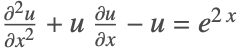
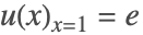
Wolfram Language code: op = Inactive[Div][{{1}}. Inactive[Grad][u[x], {x}], {x}] + u[x] * D[u[x], x] - u[x] - Exp[2 x]

解析解：

解析解を設定する．

Wolfram Language code: ares = Function[x, Exp[x]]

解析解を確かめる．

Wolfram Language code: Activate[op == 0] /. u -> ares//Simplify

境界条件：

および

境界条件を設定する．

Wolfram Language code: bcs = {NeumannValue[2 - u[x], x == 0], DirichletCondition[u[x] == E, x == 1]}

領域：

領域を設定する．

Wolfram Language code: region = Line[{{0}, {1}}]

テスト1：

非アクティブな形式の偏微分方程式をテストする．

Wolfram Language code:

VerificationTest[
	nlfun = NDSolveValue[{op == bcs[[1]], bcs[[2]]}, u, Element[{x}, region], Method -> "FiniteElement"];
	Norm[Table[nlfun[x] - ares[x], {x, 0, 1, 0.1}]] < 10 ^ -6, 
	True, 
	TestID -> "FEM-NL-Stationary-1D-Single-Convection-0002-A"
	]

テスト2：

偏微分方程式をテストする．

Wolfram Language code:

VerificationTest[
	anlfun = NDSolveValue[{Activate[op == bcs[[1]]], bcs[[2]]}, u, Element[{x}, region], Method -> "FiniteElement"];
	Norm[Table[anlfun[x] - ares[x], {x, 0, 1, 0.1}]] < 10 ^ -6, 
	True, 
	TestID -> "FEM-NL-Stationary-1D-Single-Convection-0002-B"
	]

テスト3：

低レベル関数をテストし，ステップと評価を管理する．

Wolfram Language code:

VerificationTest[
	nr = ToNumericalRegion[region];vd = NDSolve`VariableData[{"Dependent", "Space"} -> {{u}, {x}}];sd = NDSolve`SolutionData[{"Dependent", "Space"} -> {{1}, nr}];
	md = InitializePDEMethodData[vd, sd];ibcs = InitializeBoundaryConditions[vd, sd, {bcs}];
	pdec = InitializePDECoefficients[vd, sd
	, "DiffusionCoefficients" -> {{{{1}}}}
	, "ConvectionCoefficients" -> {{{{u[x]}}}}
	, "ReactionCoefficients" -> {{-1}}
	, "LoadCoefficients" -> {{Exp[2 x]}}
	];
	j = e = s = 0;
	sdNew = PDESolve[pdec, ibcs, vd, sd, md, 
	"FindRootOptions" -> {Jacobian -> {Automatic, EvaluationMonitor :> j++}, EvaluationMonitor :> e++, StepMonitor :> s++}
	];
	{eif} = ProcessPDESolutions[md, sdNew];
{Norm[Table[eif[x] - ares[x], {x, 0, 1, 0.1}]] < 10 ^ -6, e == 12, s == 11, j == 1}
	, 
	{True, True, True, True}, 
	{TestID -> "FEM-NL-Stationary-1D-Single-Convection-0002-C"}
	]

反応—FEM-NL-Stationary-1D-Single-Reaction-0001

テストの参考文献：

[1], problem 7.1, page 383.

方程式：

非アクティブな形式で方程式を設定する．

Wolfram Language code: op = Inactive[Plus][Inactive[Div][{{-1}}. Inactive[Grad][u[x], {x}], {x}], u[x] ^ 3]

解析解：

なし

境界条件：

および

境界条件を設定する．

Wolfram Language code: bcs = {DirichletCondition[u[x] == 1 / 27, x == 0], NeumannValue[5 / 3, x == 2]}

領域：

領域を設定する．

Wolfram Language code: region = Line[{{0}, {2}}]

別の数値解：

別の数値解を設定する．

Wolfram Language code: nres = NDSolveValue[{op == 0//Activate, u[0] == 1 / 27, u'[2] == 5 / 3}, u, {x, 0, 2}, Method -> "Shooting"]

テスト1：

非アクティブな形式の偏微分方程式をテストする．

Wolfram Language code:

VerificationTest[
	nlfun = NDSolveValue[{op == bcs[[2]], bcs[[1]]}, u, Element[{x}, region], Method -> sopts, InitialSeeding -> {u[x] == 1}];
	Norm[Table[nlfun[x] - nres[x], {x, 0, 2, 0.1}]] < 10 ^ -5, 
	True, 
	TestID -> "FEM-NL-Stationary-1D-Single-Reaction-0001-A"
	]

テスト2：

偏微分方程式をテストする．

Wolfram Language code:

VerificationTest[
	aeqn = Activate[op - bcs[[2]] == 0];anlfun = NDSolveValue[{aeqn, bcs[[1]]}, u, Element[{x}, region], Method -> sopts, InitialSeeding -> {u[x] == 1}];
	Norm[Table[anlfun[x] - nres[x], {x, 0, 1, 0.1}]] < 10 ^ -5, 
	True, 
	TestID -> "FEM-NL-Stationary-1D-Single-Reaction-0001-B"
	]

テスト3：

低レベル関数をテストし，ステップと評価を管理する．

Wolfram Language code:

VerificationTest[
	vd = NDSolve`VariableData[{"Dependent", "Space"} -> {{u}, {x}}];
	nr = ToNumericalRegion[region];
	sd = NDSolve`SolutionData[{"Dependent", "Space"} -> {{1}, nr}];
	md = InitializePDEMethodData[vd, sd];
	ibcs = InitializeBoundaryConditions[vd, sd, {bcs}];
	pdec = InitializePDECoefficients[vd, sd
	, "DiffusionCoefficients" -> {{{{-1}}}}
	, "ReactionCoefficients" -> {{u[x] ^ 2}}
	];
	j = e = s = 0;
	sdNew = PDESolve[pdec, ibcs, vd, sd, md, 
	"FindRootOptions" -> {Jacobian -> {Automatic, EvaluationMonitor :> j++}, EvaluationMonitor :> e++, StepMonitor :> s++}
	];
	{eif} = ProcessPDESolutions[md, sdNew];
{Norm[Table[eif[x] - nres[x], {x, 0, 1, 0.1}]] < 10 ^ -5, e == 11, s == 10, j == 1}
	, 
	{True, True, True, True}, 
	{TestID -> "FEM-NL-Stationary-1D-Single-Reaction-0001-C"}
	]

反応—FEM-NL-Stationary-1D-Single-Reaction-0002

テストの参考文献：

[1], problem 7.3, page 384.

方程式：

非アクティブな形式で方程式を設定する．

Wolfram Language code:

logTerm = (2u[x] - Log[x]) ^ 3;
op = Inactive[Plus][Inactive[Div][{{1}}. Inactive[Grad][u[x], {x}], {x}], -D[u[x], x], -logTerm]

解析解：

なし

境界条件：

および

境界条件を設定する．

Wolfram Language code: bcs = {DirichletCondition[u[x] == 1 / 2, x == 1], DirichletCondition[u[x] == 1 / 2 + Log[2], x == 2]}

領域：

領域を設定する．

Wolfram Language code: region = Line[{{1}, {2}}]

別の数値解：

別の数値解を設定する．

Wolfram Language code: nres = NDSolveValue[{op == 0//Activate, u[1] == 1 / 2, u[2] == 1 / 2 + Log[2]}, u, {x, 1, 2}]

テスト1：

非アクティブな形式の偏微分方程式をテストする．

Wolfram Language code:

VerificationTest[
	nlfun = NDSolveValue[{op == 0, bcs}, u, Element[{x}, region], Method -> sopts, InitialSeeding -> {u[x] == 1}];
	Norm[Table[nlfun[x] - nres[x], {x, 1, 2, 0.1}]] < 10 ^ -6, 
	True, 
	TestID -> "FEM-NL-Stationary-1D-Single-Reaction-0002-A"
	]

テスト2：

偏微分方程式をテストする．

Wolfram Language code:

VerificationTest[
	aeqn = Activate[op == 0];anlfun = NDSolveValue[{aeqn, bcs}, u, Element[{x}, region], Method -> sopts, InitialSeeding -> {u[x] == 1}];
	Norm[Table[anlfun[x] - nres[x], {x, 1, 2, 0.1}]] < 10 ^ -6, 
	True, 
	TestID -> "FEM-NL-Stationary-1D-Single-Reaction-0002-B"
	]

テスト3と4：

低レベル関数のデータ構造を設定する．

Wolfram Language code:

vd = NDSolve`VariableData[{"Dependent", "Space"} -> {{u}, {x}}];
nr = ToNumericalRegion[region];
sd = NDSolve`SolutionData[{"Dependent", "Space"} -> {{1}, nr}];
md = InitializePDEMethodData[vd, sd];
ibcs = InitializeBoundaryConditions[vd, sd, {bcs}];

低レベル関数をテストし，ステップと評価を管理する．

Wolfram Language code:

VerificationTest[
	pdec = InitializePDECoefficients[vd, sd
	, "DiffusionCoefficients" -> {{{{1}}}}
	, "ConvectionCoefficients" -> {{{{-1}}}}
	, "ReactionCoefficients" -> {{-6 Log[x] ^ 2 + 12 Log[x] u[x] - 8 u[x] ^ 2}}
	, "LoadCoefficients" -> {{-Log[x] ^ 3}}
	];
	j = e = s = 0;
	sdNew = PDESolve[pdec, ibcs, vd, sd, md, 
	"FindRootOptions" -> {Jacobian -> {Automatic, EvaluationMonitor :> j++}, EvaluationMonitor :> e++, StepMonitor :> s++}
	];
	{eif} = ProcessPDESolutions[md, sdNew];
{Norm[Table[eif[x] - nres[x], {x, 1, 2, 0.1}]] < 10 ^ -5, e == 11, s == 10, j == 1}
	, 
	{True, True, True, True}, 
	{TestID -> "FEM-NL-Stationary-1D-Single-Reaction-0002-C"}
	]

低レベル関数の別の形成をテストする．

Wolfram Language code:

VerificationTest[
	pdec = InitializePDECoefficients[vd, sd
	, "DiffusionCoefficients" -> {{{{1}}}}
	, "ConvectionCoefficients" -> {{{{-1}}}}
	, "LoadCoefficients" -> {{logTerm}}
	];
	j = e = s = 0;
	sdNew = PDESolve[pdec, ibcs, vd, sd, md, 
	"FindRootOptions" -> {Jacobian -> {Automatic, EvaluationMonitor :> j++}, EvaluationMonitor :> e++, StepMonitor :> s++}
	];
	{eif} = ProcessPDESolutions[md, sdNew];
{Norm[Table[eif[x] - nres[x], {x, 1, 2, 0.1}]] < 10 ^ -5, e == 11, s == 10, j == 1}
	, 
	{True, True, True, True}, 
	{TestID -> "FEM-NL-Stationary-1D-Single-Reaction-0002-D"}
	]

反応—FEM-NL-Stationary-1D-Single-Reaction-0003

テストの参考文献：

なし

方程式：

非アクティブな形式で方程式を設定する．

Wolfram Language code: op = Inactive[Plus][Inactive[Div][{{-1}}. Inactive[Grad][u[x], {x}], {x}], u[x] ^ 2]

解析解：

解析解を設定する．

Wolfram Language code:

(*ares=DSolveValue[{op==0//Activate},u,x]/.{C[1]->1,C[2]->1}*)
	ares = Function[{x}, 6^1 / 3 WeierstrassP[(x + 1) / 6^1 / 3, {0, 1}]]

境界条件：

境界条件は指定されない．境界条件は解析解から推測される．

および

境界条件を設定する．

Wolfram Language code: bcs = {DirichletCondition[u[x] == ares[0.], x == 0], DirichletCondition[u[x] == ares[1.], x == 1]}

領域：

このテストは任意領域を使う．

領域を設定する．

Wolfram Language code: region = Line[{{0}, {1}}]

テスト1：

非アクティブな形式の偏微分方程式をテストする．

Wolfram Language code:

VerificationTest[
	nlfun = NDSolveValue[{op == 0, bcs}, u, Element[{x}, region], Method -> sopts, InitialSeeding -> {u[x] == 1}];
	Norm[Table[nlfun[x] - ares[x], {x, 0, 1, 0.1}]] < 10 ^ -5, 
	True, 
	TestID -> "FEM-NL-Stationary-1D-Single-Reaction-0003-A"
	]

テスト2：

偏微分方程式をテストする．

Wolfram Language code:

VerificationTest[
	aeqn = Activate[op == 0];anlfun = NDSolveValue[{aeqn, bcs}, u, Element[{x}, region], Method -> sopts, InitialSeeding -> {u[x] == 1}];
	Norm[Table[anlfun[x] - ares[x], {x, 0, 1, 0.1}]] < 10 ^ -5, 
	True, 
	TestID -> "FEM-NL-Stationary-1D-Single-Reaction-0003-B"
	]

テスト3と4：

低レベル関数のデータ構造を設定する．

Wolfram Language code:

vd = NDSolve`VariableData[{"Dependent", "Space"} -> {{u}, {x}}];
nr = ToNumericalRegion[region];
sd = NDSolve`SolutionData[{"Dependent", "Space"} -> {{1}, nr}];
md = InitializePDEMethodData[vd, sd];
ibcs = InitializeBoundaryConditions[vd, sd, {bcs}];

低レベル関数をテストし，ステップと評価を管理する．

Wolfram Language code:

VerificationTest[
	pdec = InitializePDECoefficients[vd, sd
	, "DiffusionCoefficients" -> {{{{-1}}}}
	, "LoadCoefficients" -> {{-u[x] ^ 2}}
	];
	j = e = s = 0;
	sdNew = PDESolve[pdec, ibcs, vd, sd, md, 
	"FindRootOptions" -> {Jacobian -> {Automatic, EvaluationMonitor :> j++}, EvaluationMonitor :> e++, StepMonitor :> s++}
	];
	{eif} = ProcessPDESolutions[md, sdNew];
{Norm[Table[eif[x] - ares[x], {x, 0, 1, 0.1}]] < 10 ^ -5, e == 10, s == 9, j == 1}
	, 
	{True, True, True, True}, 
	{TestID -> "FEM-NL-Stationary-1D-Single-Reaction-0003-C"}
	]

低レベル関数の別の定式化をテストする．

Wolfram Language code:

VerificationTest[
	pdec = InitializePDECoefficients[vd, sd
	, "DiffusionCoefficients" -> {{{{-1}}}}
	, "ReactionCoefficients" -> {{u[x]}}
	];
	j = e = s = 0;
	sdNew = PDESolve[pdec, ibcs, vd, sd, md, 
	"FindRootOptions" -> {Jacobian -> {Automatic, EvaluationMonitor :> j++}, EvaluationMonitor :> e++, StepMonitor :> s++}
	];
	{eif} = ProcessPDESolutions[md, sdNew];
{Norm[Table[eif[x] - ares[x], {x, 0, 1, 0.1}]] < 10 ^ -5, e == 10, s == 9, j == 1}
	, 
	{True, True, True, True}, 
	{TestID -> "FEM-NL-Stationary-1D-Single-Reaction-0003-D"}
	]

反応—FEM-NL-Stationary-1D-Single-Reaction-0004

テストの参考文献：

なし

方程式：

非アクティブな形式で方程式を設定する．

Wolfram Language code: op = Inactive[Plus][Inactive[Div][{{-1}}. Inactive[Grad][u[x], {x}], {x}], I u[x] ^ 2]

解析解：

-(-1)^5/6

解析解を設定する．

Wolfram Language code:

(*ares=DSolveValue[{op==0//Activate},u,x]/.{C[1]->1,C[2]->1}*)
	ares = Function[{x}, -(-1)^5 / 6 6^1 / 3 WeierstrassP[((-1)^1 / 6 (x + 1)/6^1 / 3), {0, 1}]]

境界条件：

境界条件は指定されない．境界条件は解析解から推測される．

および

境界条件を設定する．

Wolfram Language code: bcs = {DirichletCondition[u[x] == ares[0.], x == 0], DirichletCondition[u[x] == ares[1.], x == 1]}

領域：

このテストは任意領域を使う．

領域を設定する．

Wolfram Language code: region = Line[{{0}, {1}}]

テスト1：

非アクティブな形式の偏微分方程式をテストする．

Wolfram Language code:

VerificationTest[
	nlfun = NDSolveValue[{op == 0, bcs}, u, Element[{x}, region], Method -> sopts, InitialSeeding -> {u[x] == 1}];
	Norm[Table[nlfun[x] - ares[x], {x, 0, 1, 0.1}]] < 10 ^ -5, 
	True, 
	TestID -> "FEM-NL-Stationary-1D-Single-Reaction-0004-A"
	]

テスト2：

偏微分方程式をテストする．

Wolfram Language code:

VerificationTest[
	aeqn = Activate[op == 0];anlfun = NDSolveValue[{aeqn, bcs}, u, Element[{x}, region], Method -> sopts, InitialSeeding -> {u[x] == 1}];
	Norm[Table[anlfun[x] - ares[x], {x, 0, 1, 0.1}]] < 10 ^ -5, 
	True, 
	TestID -> "FEM-NL-Stationary-1D-Single-Reaction-0004-B"
	]

テスト3と4：

低レベル関数のデータ構造を設定する．

Wolfram Language code:

vd = NDSolve`VariableData[{"Dependent", "Space"} -> {{u}, {x}}];
nr = ToNumericalRegion[region];
sd = NDSolve`SolutionData[{"Dependent", "Space"} -> {{1}, nr}];
md = InitializePDEMethodData[vd, sd];
ibcs = InitializeBoundaryConditions[vd, sd, {bcs}];

低レベル関数をテストし，ステップと評価を管理する．

Wolfram Language code:

VerificationTest[
	pdec = InitializePDECoefficients[vd, sd
	, "DiffusionCoefficients" -> {{{{-1}}}}
	, "LoadCoefficients" -> {{-I u[x] ^ 2}}
	];
	j = e = s = 0;
	sdNew = PDESolve[pdec, ibcs, vd, sd, md, 
	"FindRootOptions" -> {Jacobian -> {Automatic, EvaluationMonitor :> j++}, EvaluationMonitor :> e++, StepMonitor :> s++}
	];
	{eif} = ProcessPDESolutions[md, sdNew];
{Norm[Table[eif[x] - ares[x], {x, 0, 1, 0.1}]] < 10 ^ -5, e == 13, s == 11, j == 2}
	, 
	{True, True, True, True}, 
	{TestID -> "FEM-NL-Stationary-1D-Single-Reaction-0004-C"}
	]

低レベル関数の別の定式化をテストする．

Wolfram Language code:

VerificationTest[
	pdec = InitializePDECoefficients[vd, sd
	, "DiffusionCoefficients" -> {{{{-1}}}}
	, "ReactionCoefficients" -> {{I u[x]}}
	];
	j = e = s = 0;
	sdNew = PDESolve[pdec, ibcs, vd, sd, md, 
	"FindRootOptions" -> {Jacobian -> {Automatic, EvaluationMonitor :> j++}, EvaluationMonitor :> e++, StepMonitor :> s++}
	];
	{eif} = ProcessPDESolutions[md, sdNew];
{Norm[Table[eif[x] - ares[x], {x, 0, 1, 0.1}]] < 10 ^ -5, e == 13, s == 11, j == 2}
	, 
	{True, True, True, True}, 
	{TestID -> "FEM-NL-Stationary-1D-Single-Reaction-0004-D"}
	]

負荷—FEM-NL-Stationary-1D-Single-Load-0001

テストの参考文献：

[3], Exact Solutions > Ordinary Differential Equations > Second-Order Nonlinear Ordinary Differential Equations; Equation 3.1.1; Autonomous equation.

方程式：

非アクティブな形式で方程式を設定する．

Wolfram Language code: op = Inactive[Div][{{1}}. Inactive[Grad][u[x], {x}], {x}] - Sin[u[x]]

解析解：

このとき，C₁ と C₂ は任意定数である．

解析解を設定する．

Wolfram Language code:

(*temp=Integrate[(C[1]+2*Integrate[Sin[u[x]],u[x]])^(-1/2),u[x]]==C[2]+x/.{C[1]->3,C[2]->3};
ares=Function[x,Evaluate[(u[x]/.Solve[temp,u[x]])[[1]]]]*)
ares = Function[x, 2 JacobiAmplitude[(3 + x/2), -4]]

解析解を確かめる．

Wolfram Language code: Activate[op == 0] /. u -> ares//Simplify

境界条件：

境界条件は指定されない．境界条件は解析解から推測される．

および

境界条件を設定する．

Wolfram Language code: bcs = {DirichletCondition[u[x] == ares[0.], x == 0], DirichletCondition[u[x] == ares[1.], x == 1]}

領域：

このテストは任意領域を使う．

領域を設定する．

Wolfram Language code: region = Line[{{0}, {1}}]

テスト1：

非アクティブな形式の偏微分方程式をテストする．

Wolfram Language code:

VerificationTest[
	aeqn = Activate[op == 0];anlfun = NDSolveValue[{aeqn, bcs}, u, Element[{x}, region], Method -> sopts, InitialSeeding -> {u[x] == 1}];
	Norm[Table[anlfun[x] - ares[x], {x, 0, 1, 0.1}]] < 10 ^ -9, 
	True, 
	TestID -> "FEM-NL-Stationary-1D-Single-Load-0001-B"
	]

テスト2：

偏微分方程式をテストする．

Wolfram Language code:

VerificationTest[
	aeqn = Activate[op == 0];anlfun = NDSolveValue[{aeqn, bcs}, u, Element[{x}, region], Method -> sopts, InitialSeeding -> {u[x] == 1}];
	Norm[Table[anlfun[x] - ares[x], {x, 0, 1, 0.1}]] < 10 ^ -9, 
	True, 
	TestID -> "FEM-NL-Stationary-1D-Single-Load-0001-B"
	]

テスト3：

低レベル関数をテストし，ステップと評価を管理する．

Wolfram Language code:

VerificationTest[
	vd = NDSolve`VariableData[{"Dependent", "Space"} -> {{u}, {x}}];
	nr = ToNumericalRegion[region];
	sd = NDSolve`SolutionData[{"Dependent", "Space"} -> {{1}, nr}];
	md = InitializePDEMethodData[vd, sd];
	ibcs = InitializeBoundaryConditions[vd, sd, {bcs}];
	pdec = InitializePDECoefficients[vd, sd
	, "DiffusionCoefficients" -> {{{{1}}}}
	, "LoadCoefficients" -> {{Sin[u[x]]}}
	];
	j = e = s = 0;
	sdNew = PDESolve[pdec, ibcs, vd, sd, md, 
	"FindRootOptions" -> {Jacobian -> {Automatic, EvaluationMonitor :> j++}, EvaluationMonitor :> e++, StepMonitor :> s++}
	];
	{eif} = ProcessPDESolutions[md, sdNew];
{Norm[Table[eif[x] - ares[x], {x, 0, 1, 0.1}]] < 10 ^ -9, e == 8, s == 7, j == 1}
	, 
	{True, True, True, True}, 
	{TestID -> "FEM-NL-Stationary-1D-Single-Load-0001-C"}
	]

負荷—FEM-NL-Stationary-1D-Single-Load-0002

テストの参考文献：

[2], problem 3.17, page 84.

方程式：

非アクティブな形式で方程式を設定する．

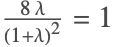
Wolfram Language code: op = Inactive[Div][{{-x}}. Inactive[Grad][u[x], {x}], {x}] - x Exp[u[x]]

解析解：

（）

このとき λ_i は方程式の根である．

解析解を設定する．

Wolfram Language code:

(*params=Solve[8*λ/(1+λ)^2==1,λ]*)
	params = {{λ -> 3 - 2 * Sqrt[2]}, {λ -> 3 + 2 * Sqrt[2]}};
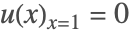
	ares = Function[x, Log[8 * λ / (1 + λ * x ^ 2) ^ 2]] /. params

境界条件：

および

境界条件を設定する．

Wolfram Language code: bcs = {DirichletCondition[u[x] == 0, x == 1]}

領域：

このテストは任意領域を使う．

領域を設定する．

Wolfram Language code: region = Line[{{0}, {1}}]

テスト1：

初期シード値で非アクティブな偏微分方程式をテストし，解を1つ得る．

Wolfram Language code:

VerificationTest[
	nlfun = NDSolveValue[{op == 0, bcs}, u, Element[{x}, region], Method -> sopts, InitialSeeding -> {u[x] == 1}];
	Norm[Table[nlfun[x] - ares[[1]][x], {x, 0, 1, 0.1}]] < 10 ^ -7, 
	True, 
	TestID -> "FEM-NL-Stationary-1D-Single-Load-0002-A"
	]

テスト2：

別の初期シード値で非アクティブな偏微分方程式をテストし，別の解を1つ得る．

Wolfram Language code:

VerificationTest[
	nlfun = NDSolveValue[{op == 0, bcs}, u, Element[{x}, region], Method -> sopts, InitialSeeding -> {u[x] == -4x + 4}];
	Norm[Table[nlfun[x] - ares[[2]][x], {x, 0, 1, 0.1}]] < 10 ^ -4, 
	True, 
	TestID -> "FEM-NL-Stationary-1D-Single-Load-0002-B"
	]

テスト3：

偏微分方程式をテストする．

Wolfram Language code:

VerificationTest[
	aeqn = Activate[op == 0];anlfun = NDSolveValue[{aeqn, bcs}, u, Element[{x}, region], Method -> sopts, InitialSeeding -> {u[x] == 1}];
	Norm[Table[anlfun[x] - ares[[1]][x], {x, 0, 1, 0.1}]] < 10 ^ -7, 
	True, 
	TestID -> "FEM-NL-Stationary-1D-Single-Load-0002-C"
	]

テスト4：

別の初期シード値でアクティブな偏微分方程式をテストし，別の解を1つ得る．

Wolfram Language code:

VerificationTest[
	aeqn = Activate[op == 0];anlfun = NDSolveValue[{aeqn, bcs}, u, Element[{x}, region], Method -> sopts, InitialSeeding -> {u[x] == -4x + 4}];
	Norm[Table[anlfun[x] - ares[[2]][x], {x, 0, 1, 0.1}]] < 10 ^ -4, 
	True, 
	TestID -> "FEM-NL-Stationary-1D-Single-Load-0002-D"
	]

放射境界条件—FEM-NL-Stationary-1D-Single-Radiation-0001

テストの参考文献：

[1], problem 7.13, page 385.

モデル問題を修正し，比較のために解析解が使えるようにし，非線形境界条件のテストを拡張する．

方程式：

[1]で与えられたパラメータを2つの点において変更する．まず，T_∞ に非零の値を与えて，テストのスコープを拡張する．次に，P を0に設定して解析解が使えるようにする．

パラメータを指定する．

Wolfram Language code:

params = {k -> 40, σ -> 5675 / 1000 * 10 ^ -8, ϵpsi -> 35 / 100, q -> 0, len -> 4 / 10, T0 -> 500, TInf -> 100, A -> π * radius ^ 2, P -> 0} /. radius -> 5 / 1000;

非アクティブな形式で方程式を設定する．

Wolfram Language code: op = Inactive[Div][{{-k * A}}. Inactive[Grad][u[x], {x}], {x}] /. params

解析解：

位置 L では，u の解は以下のように求まる（その下に微分を示す）．

L の解．

Wolfram Language code: aresL = Root[-4000158900000000 + 8000000000000 #1 + 1589 #1^4&, 2]

以下は，L における解の微分である．テストの実行時に時間がかからないように，セルは評価できないようになっている．

一般解の構造は以下の通りである．

Wolfram Language code: tfun = DSolveValue[Activate[op == 0], u, x]

以下に注意する．

Wolfram Language code: c2 = Integrate[D[u[x], {x, 2}], x] -> C[2]

x=0においてDirichletConditionによって示唆される第1制約条件を指定する．

Wolfram Language code: c1 = tfun[0] -> T0 /. params

c₂から示唆される第2制約条件を指定する．

Wolfram Language code: c3 = Solve[u[x] == tfun[x] /. x -> len /. params, C[2]]

一般化されたノイマン値の定義を使い，制約条件を挿入する．

Wolfram Language code:

eqn = k A D[u[x], x] == -ϵpsi * σ * A * (u[len] ^ 4 - TInf ^ 4) //. 
	Flatten[{c1, c2, c3}] /. params

Reduceを使って正の実根を求める．

Wolfram Language code: Reduce[{eqn, u[len] > 0} /. params, {u[len]} /. params, Reals]

境界条件：

および

境界条件を設定する．

Wolfram Language code: bcs = {DirichletCondition[u[x] == T0, x == 0], NeumannValue[ -ϵpsi * σ * A(u[x] ^ 4 - TInf ^ 4), x == len]} /. params

領域：

このテストは任意領域を使う．

領域を設定する．

Wolfram Language code: region = Line[{{0}, {len}}] /. params

テスト1：

初期シード値で非アクティブな偏微分方程式をテストし，解を1つ得る．

Wolfram Language code:

VerificationTest[
	nlfun = NDSolveValue[{op == bcs[[2]], bcs[[1]]}, u, Element[{x}, region], Method -> sopts, InitialSeeding -> {u[x] == 1}];
	(nlfun[len] /. params) - aresL < 10 ^ -12, 
	True, 
	TestID -> "FEM-NL-Stationary-1D-Single-Radiation-0001-A"
	]

テスト2：

初期シード値でアクティブな偏微分方程式をテストし，解を1つ得る．

Wolfram Language code:

VerificationTest[
	nlfun = NDSolveValue[{Activate[op == bcs[[2]]], bcs[[1]]}, u, Element[{x}, region], Method -> sopts, InitialSeeding -> {u[x] == 1}];
	(nlfun[len] /. params) - aresL < 10 ^ -12, 
	True, 
	TestID -> "FEM-NL-Stationary-1D-Single-Radiation-0001-B"
	]

テスト3：

低レベル関数をテストし，ステップと評価を管理する．

Wolfram Language code:

VerificationTest[
	vd = NDSolve`VariableData[{"Dependent", "Space"} -> {{u}, {x}}];
	nr = ToNumericalRegion[region];
	sd = NDSolve`SolutionData[{"Dependent", "Space"} -> {{1}, nr}];
	md = InitializePDEMethodData[vd, sd];
	ibcs = InitializeBoundaryConditions[vd, sd, {bcs}];
	pdec = InitializePDECoefficients[vd, sd
	, "DiffusionCoefficients" -> {{{{-k A}}}} /. params
	];
	j = e = s = 0;
	sdNew = PDESolve[pdec, ibcs, vd, sd, md, 
	"FindRootOptions" -> {Jacobian -> {Automatic, EvaluationMonitor :> j++}, EvaluationMonitor :> e++, StepMonitor :> s++}
	];
	{eif} = ProcessPDESolutions[md, sdNew];
{(eif[len] /. params) - aresL < 10 ^ -12, e == 8, s == 7, j == 1}
	, 
	{True, True, True, True}, 
	{TestID -> "FEM-NL-Stationary-1D-Single-Load-0001-C"}
	]

一次元方程式系

このセクションには，非線形の常微分方程式系の例が含まれる．

反応—FEM-NL-Stationary-1D-System-Reaction-0001

テストの参考文献：

[3], Exact Solutions > Systems of Ordinary Differential Equations > Nonlinear Systems of Two Ordinary Differential Equations, 3.2.7

方程式：

f と g の特定値について方程式を設定する．

Wolfram Language code:

ClearAll[f, g]
rls = {f -> Sin, g -> Cos};
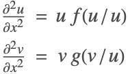
op = {Inactive[Plus][Inactive[Div][Inactive[Grad][u[x], {x}], {x}], -u[x] * f[v[x] / u[x]] ], 
	Inactive[Plus][Inactive[Div][Inactive[Grad][v[x], {x}], {x}], -v[x] * g[v[x] / u[x]] ]
	} /. rls

解析解：

解析解を設定する．

Wolfram Language code:

ClearAll[k]
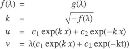
params = Flatten[{FindRoot[f[λ] == g[λ] /. rls//Evaluate, {λ, 1 / 2}], 
k -> Sqrt[f[λ]] /. rls, C[1] -> 1, C[2] -> 2}];
ares = Function[x, Evaluate[(C[1] * Exp[k * x] + C[2] * Exp[-k * x]) //. params]]
bres = Function[x, Evaluate[(λ * (C[1] * Exp[k * x] + C[2] * Exp[-k * x]) //. params)]]

境界条件：

境界条件は指定されない．境界条件は解析解から推測される．

境界条件を設定する．

Wolfram Language code:

bcs = {{DirichletCondition[u[x] == ares[0], x == 0], DirichletCondition[u[x] == ares[1], x == 1]}, {DirichletCondition[v[x] == bres[0], x == 0], DirichletCondition[v[x] == bres[1], x == 1]}} //. params

領域：

領域を設定する．

Wolfram Language code: region = Line[{{0}, {1}}]

テスト1：

非アクティブな形式の偏微分方程式をテストする．

Wolfram Language code:

VerificationTest[
	{nlfun1, nlfun2} = NDSolveValue[{op == {0, 0}, bcs}, {u, v}, Element[{x}, region], Method -> sopts, InitialSeeding -> {u[x] == 1, v[x] == x}];
	{Norm[Table[nlfun1[x] - ares[x], {x, 0, 1, 0.1}]] < 10 ^ -8, Norm[Table[nlfun2[x] - bres[x], {x, 0, 1, 0.1}]] < 10 ^ -8}, 
	{True, True}, 
	TestID -> "FEM-NL-Stationary-1D-System-Reaction-0001-A"
	]

テスト2：

偏微分方程式をテストする．

Wolfram Language code:

VerificationTest[
	{anlfun1, anlfun2} = NDSolveValue[{Activate[op == {0, 0}], bcs}, {u, v}, Element[{x}, region], Method -> sopts, InitialSeeding -> {u[x] == 1, v[x] == x}];
	{Norm[Table[anlfun1[x] - ares[x], {x, 0, 1, 0.1}]] < 10 ^ -8, Norm[Table[anlfun2[x] - bres[x], {x, 0, 1, 0.1}]] < 10 ^ -8}
	, 
	{True, True}, 
	TestID -> "FEM-NL-Stationary-1D-System-Reaction-0001-B"
	]

テスト3と4：

低レベル関数のデータ構造を設定する．

Wolfram Language code:

vd = NDSolve`VariableData[{"Dependent", "Space"} -> {{u, v}, {x}}];
nr = ToNumericalRegion[region];
sd = NDSolve`SolutionData[{"Dependent", "Space"} -> {{1, x}, nr}];
md = InitializePDEMethodData[vd, sd];
ibcs = InitializeBoundaryConditions[vd, sd, bcs];

低レベル関数をテストし，ステップと評価を管理する．

Wolfram Language code:

VerificationTest[
	pdec = InitializePDECoefficients[vd, sd
	, "DiffusionCoefficients" -> {{{{1}}, {{0}}}, {{{0}}, {{1}}}}
	, "ReactionCoefficients" -> {{-Sin[v[x] / u[x]], 0}, {0, -Cos[v[x] / u[x]]}}
	];
	j = e = s = 0;
	sdNew = PDESolve[pdec, ibcs, vd, sd, md, 
	"FindRootOptions" -> {Jacobian -> {Automatic, EvaluationMonitor :> j++}, EvaluationMonitor :> e++, StepMonitor :> s++}
	];
	{eif1, eif2} = ProcessPDESolutions[md, sdNew];
{Norm[Table[eif1[x] - ares[x], {x, 0, 1, 0.1}]] < 10 ^ -8, Norm[Table[eif2[x] - bres[x], {x, 0, 1, 0.1}]] < 10 ^ -8, e == 7, s == 6, j == 1}
	, 
	{True, True, True, True, True}, 
	{TestID -> "FEM-NL-Stationary-1D-System-Reaction-0001-C"}
	]

低レベル関数の別の定式化をテストする．

Wolfram Language code:

VerificationTest[
	pdec = InitializePDECoefficients[vd, sd
	, "DiffusionCoefficients" -> {{{{1}}, {{0}}}, {{{0}}, {{1}}}}
	, "LoadCoefficients" -> {{Sin[v[x] / u[x]] * u[x]}, {Cos[v[x] / u[x]] * v[x]}}
	];
	j = e = s = 0;
	sdNew = PDESolve[pdec, ibcs, vd, sd, md, 
	"FindRootOptions" -> {Jacobian -> {Automatic, EvaluationMonitor :> j++}, EvaluationMonitor :> e++, StepMonitor :> s++}
	];
	{eif1, eif2} = ProcessPDESolutions[md, sdNew];
{Norm[Table[eif1[x] - ares[x], {x, 0, 1, 0.1}]] < 10 ^ -8, Norm[Table[eif2[x] - bres[x], {x, 0, 1, 0.1}]] < 10 ^ -8, e == 7, s == 6, j == 1}
	, 
	{True, True, True, True, True}, 
	{TestID -> "FEM-NL-Stationary-1D-System-Reaction-0001-D"}
	]

二次元の単一方程式

このセクションには，単一方程式を含む非線形の偏微分方程式の例が含まれる．

拡散—FEM-NL-Stationary-2D-Single-Diffusion-0001

テストの参考文献：

[3], Exact Solutions > Nonlinear Partial Differential Equations > Other Second-Order Partial Differential Equations; Equation 4.1.2; Equation of steady transonic gas flow.

方程式：

非アクティブな形式で方程式を設定する．

Wolfram Language code:

op = Inactive[Plus][Inactive[Div][{{b D[u[x, y], x], 0}, {0, 1}}. Inactive[Grad][u[x, y], {x, y}], {x, y}], a / y D[u[x, y], y]]

解析解：

任意定数 C[1]，C[2]，C[3]，C[4]，a， b で解析解を設定する．

Wolfram Language code:

params = {C[1] -> 1, C[2] -> 1, C[3] -> 1, C[4] -> 1, a -> 1, b -> 1};
ares = Function[{x, y}, Evaluate[-(b C[1]) / (2(a + 1)) y ^ 2 + C[2]y ^ (1 - a) + C[3] + 2 / (3 C[1])(C[1]x + C[4]) ^ (3 / 2) /. params]]

解析解を検証する．

Wolfram Language code: Activate[op /. u -> ares /. params]

境界条件：

境界条件は指定されない．境界条件は解析解から推測される．

境界条件を設定する．

Wolfram Language code: bcs = {DirichletCondition[u[x, y] == ares[x, y], True]}

領域：

領域を設定する．

Wolfram Language code: region = Rectangle[{1, 1}, {2, 3}]

テスト1：

非アクティブな形式の偏微分方程式をテストする．

Wolfram Language code:

VerificationTest[
	nlfun = NDSolveValue[{op == 0, bcs} /. params, u, Element[{x, y}, region], Method -> sopts, InitialSeeding -> {u[x, y] == 2 + Sqrt[2] / 3 + Sqrt[2] * x - y ^ 2 / 4}];
	Norm[Table[nlfun[x, y] - ares[x, y], {x, 1, 2, 0.1}, {y, 1, 3, 0.1}]] < 10 ^ -4, 
	True, 
	TestID -> "FEM-NL-Stationary-2D-Single-Diffusion-0001-A"
	]

テスト2：

アクティベートされたものの場合は，線形化の結果，偏微分方程式の係数で一次微分よりも高次の微分になり，これは処理することができない．

偏微分方程式をテストする．

Wolfram Language code:

VerificationTest[
	anlfun = NDSolveValue[{Activate[op] == 0, bcs} /. params, u, Element[{x, y}, region], Method -> sopts, InitialSeeding -> {u[x, y] == 2 + Sqrt[2] / 3 + Sqrt[2] * x - y ^ 2 / 4}];
	Head[anlfun] === NDSolveValue, 
	True, 
	NDSolveValue::femnlmdor, 
	TestID -> "FEM-NL-Stationary-2D-Single-Diffusion-0001-B"
	]

テスト3：

低レベル関数のデータ構造を設定する．

Wolfram Language code:

vd = NDSolve`VariableData[{"Dependent", "Space"} -> {{u}, {x, y}}];
nr = ToNumericalRegion[region];
sd = NDSolve`SolutionData[{"Dependent", "Space"} -> {{2 + Sqrt[2] / 3 + Sqrt[2] * x - y ^ 2 / 4}, nr}];
md = InitializePDEMethodData[vd, sd];
ibcs = InitializeBoundaryConditions[vd, sd, {bcs}];

低レベル関数をテストし，ステップと評価を管理する．

Wolfram Language code:

VerificationTest[
	pdec = InitializePDECoefficients[vd, sd
	, "DiffusionCoefficients" -> {{{{b D[u[x, y], x], 0}, {0, 1}}}} /. params
	, "ConvectionCoefficients" -> {{{{0, a / y}}}} /. params
	];
	j = e = s = 0;
	sdNew = PDESolve[pdec, ibcs, vd, sd, md, 
	"FindRootOptions" -> {Jacobian -> {Automatic, EvaluationMonitor :> j++}, EvaluationMonitor :> e++, StepMonitor :> s++}
	];
	{eif} = ProcessPDESolutions[md, sdNew];{Norm[Table[eif[x, y] - ares[x, y], {x, 1, 2, 0.1}, {y, 1, 3, 0.1}]] < 10 ^ -4, e == 16, s == 14, j == 2}
	, 
	{True, True, True, True}, 
	{TestID -> "FEM-NL-Stationary-2D-Single-Diffusion-0001-C"}
	]

反応—FEM-NL-Stationary-2D-Single-Reaction-0001

テストの参考文献：

[3], Exact Solutions > Nonlinear Partial Differential Equations > Second-Order Elliptic Partial Differential Equations; Equation 3.1.2;

方程式：

非アクティブな形式で方程式を設定する．

Wolfram Language code:

rls = {a -> -1, b -> 2, n -> 2};
op = Inactive[Plus][Inactive[Div][-{{1, 0}, {0, 1}}. Inactive[Grad][u[x, y], {x, y}], {x, y}], a u[x, y] ^ n, b u[x, y] ^ (2 * n - 1)] /. rls

解析解：

任意定数 C[1]と C[1]で解析解を設定する．

Wolfram Language code:

rls2 = {C[1] -> π / 4, C[2] -> -1};
ares = Function[{x, y}, Evaluate[((a * (1 - n) ^ 2 / (2 * (n + 1))) * (x * Sin[C[1]] + y * Cos[C[1]] + C[2]) ^ 2 - (b * (n + 1)) / (2 * a * n)) ^ (1 / (1 - n)) /. Flatten[{rls, rls2}]]]

境界条件：

境界条件は指定されない．境界条件は解析解から推測される．

境界条件を設定する．

Wolfram Language code: bcs = {DirichletCondition[u[x, y] == ares[x, y], True]}

領域：

領域を設定する．

Wolfram Language code: region = Rectangle[{-1, -1}, {1, 1}]

テスト1：

非アクティブな形式の偏微分方程式をテストする．

Wolfram Language code:

VerificationTest[
	nlfun = NDSolveValue[{op == 0, bcs}, u, Element[{x, y}, region], Method -> sopts];
	Norm[Table[nlfun[x, y] - ares[x, y], {x, -1, 1, 0.1}, {y, -1, 1, 0.1}]] < 10 ^ -4, 
	True, 
	TestID -> "FEM-NL-Stationary-2D-Single-Reaction-0001-A"
	]

テスト2：

偏微分方程式をテストする．

Wolfram Language code:

VerificationTest[
	anlfun = NDSolveValue[{Activate[op == 0], bcs}, u, Element[{x, y}, region], Method -> sopts];
	Norm[Table[anlfun[x, y] - ares[x, y], {x, -1, 1, 0.1}, {y, -1, 1, 0.1}]] < 10 ^ -4, 
	True, 
	TestID -> "FEM-NL-Stationary-2D-Single-Reaction-0001-B"
	]

テスト3と4：

低レベル関数のデータ構造を設定する．

Wolfram Language code:

vd = NDSolve`VariableData[{"Dependent", "Space"} -> {{u}, {x, y}}];
nr = ToNumericalRegion[region];
sd = NDSolve`SolutionData[{"Dependent", "Space"} -> {{1}, nr}];
md = InitializePDEMethodData[vd, sd];
ibcs = InitializeBoundaryConditions[vd, sd, {bcs}];

低レベル関数をテストし，ステップと評価を管理する．

Wolfram Language code:

VerificationTest[
	pdec = InitializePDECoefficients[vd, sd
	, "DiffusionCoefficients" -> {{{{-1, 0}, {0, -1}}}}
	, "ReactionCoefficients" -> {{(a u[x, y] ^ n + b u[x, y] ^ (2 * n - 1)) / u[x, y]}} /. rls
	];
	j = e = s = 0;
	sdNew = PDESolve[pdec, ibcs, vd, sd, md, 
	"FindRootOptions" -> {Jacobian -> {Automatic, EvaluationMonitor :> j++}, EvaluationMonitor :> e++, StepMonitor :> s++}
	];
	{eif} = ProcessPDESolutions[md, sdNew];{Norm[Table[eif[x, y] - ares[x, y], {x, -1, 1, 0.1}, {y, -1, 1, 0.1}]] < 10 ^ -4, e == 10, s == 9, j == 1}
	, 
	{True, True, True, True}, 
	{TestID -> "FEM-NL-Stationary-2D-Single-Reaction-0001-C"}
	]

低レベル関数の別の定式化をテストする．

Wolfram Language code:

VerificationTest[
	pdec = InitializePDECoefficients[vd, sd
	, "DiffusionCoefficients" -> {{{{-1, 0}, {0, -1}}}}
	, "LoadCoefficients" -> {-{a u[x, y] ^ n + b u[x, y] ^ (2 * n - 1)}} /. rls
	];
	j = e = s = 0;
	sdNew = PDESolve[pdec, ibcs, vd, sd, md, 
	"FindRootOptions" -> {Jacobian -> {Automatic, EvaluationMonitor :> j++}, EvaluationMonitor :> e++, StepMonitor :> s++}
	];
	{eif} = ProcessPDESolutions[md, sdNew];{Norm[Table[eif[x, y] - ares[x, y], {x, -1, 1, 0.1}, {y, -1, 1, 0.1}]] < 10 ^ -4, e == 10, s == 9, j == 1}
	, 
	{True, True, True, True}, 
	{TestID -> "FEM-NL-Stationary-2D-Single-Reaction-0001-D"}
	]

非定常テスト

このセクションには，テストに使うための，時間に依存する非線形偏微分方程式が含まれる．

一次元の単一方程式

このセクションには，単一方程式を含む時間依存の非線形常微分方程式の例が含まれる．独立変数が1つである常微分方程式は，通常は2つ以上の独立変数を扱う偏微分方程式の特別な場合である．

拡散—FEM-NL-Transient-1D-Single-Diffusion-0001

テストの参考文献：

[3], Exact Solutions > Nonlinear Partial Differential Equations >Second-Order Parabolic Partial Differential Equations > Heat Equation with a Power-Law Nonlinearity; Equation 1.2.1; Heat equation with a power-law nonlinearity.

方程式：

非アクティブな形式で方程式を設定する．

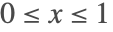
Wolfram Language code: op = D[u[t, x], t] + a Inactive[Div][{{-u[t, x]^m}}. Inactive[Grad][u[t, x], {x}], {x}]

解析解：

解のパラメータを設定する．

Wolfram Language code: params = {a -> 2, λ -> 3, m -> 3}

解析解を設定する．

Wolfram Language code: ares = Function[{t, x}, Evaluate[(λ m / a x + λ m / a λ t + 1) ^ (1 / m) /. params]]

境界条件：

境界条件は指定されない．境界条件は解析解から推測される．

および

境界条件を設定する．

Wolfram Language code: bcs = {DirichletCondition[u[t, x] == ares[t, x], True]}

初期条件：

初期条件は指定されない．初期条件は解析解から推測される．

初期条件を設定する．

Wolfram Language code: ics = {u[0, x] == ares[0, x]}

領域：

領域を設定する．

Wolfram Language code: region = Line[{{0}, {1}}]

テスト1：

非アクティブな形式の偏微分方程式をテストする．

Wolfram Language code:

VerificationTest[
	nlfun = NDSolveValue[{op == 0, bcs, ics} /. params, u, {t, 0, 1}, Element[{x}, region], Method -> topts];
	Norm[Table[nlfun[t, x] - ares[t, x] /. params, {t, 0, 1, 0.1}, {x, 0, 1, 0.1}]] < 10 ^ -2, 
	True, 
	TestID -> "FEM-NL-Transient-1D-Single-Diffusion-0001-A"
	]

テスト2：

偏微分方程式をテストする．

Wolfram Language code:

VerificationTest[
	aeqn = Activate[{op == 0, bcs, ics} /. params];
	anlfun = NDSolveValue[aeqn, u, {t, 0, 1}, Element[{x}, region], Method -> topts];
	Norm[Table[anlfun[t, x] - ares[t, x], {t, 0, 1, 0.1}, {x, 0, 1, 0.1}]] < 10 ^ -2, 
	True, 
	TestID -> "FEM-NL-Transient-1D-Single-Diffusion-0001-B"
	]

拡散—FEM-NL-Transient-1D-Single-Diffusion-0002

テストの参考文献：

[3], Exact Solutions > Nonlinear Partial Differential Equations >Second-Order Parabolic Partial Differential Equations > Heat Equation with a Exponential Nonlinearity; Equation 1.2.7; Heat Equation with a Exponential Nonlinearity.

方程式：

非アクティブな形式で方程式を設定する．

Wolfram Language code: op = D[u[t, x], t] + a Inactive[Div][{{-Exp[λ u[t, x]]}}. Inactive[Grad][u[t, x], {x}], {x}]

解析解：

解のパラメータを設定する．

Wolfram Language code: params = {A -> 1, B -> 2, λ -> 3, a -> 1 / 2}

解析解を設定する．

Wolfram Language code: ares = Function[{t, x}, Evaluate[2 / λ Log[(x + A) / Sqrt[B - 2 a t]] /. params]]

境界条件：

境界条件は指定されない．境界条件は解析解から推測される．

および

境界条件を設定する．

Wolfram Language code: bcs = {DirichletCondition[u[t, x] == ares[t, x], True]}

初期条件：

初期条件は指定されない．初期条件は解析解から推測される．

初期条件を設定する．

Wolfram Language code: ics = {u[0, x] == ares[0, x]}

領域：

領域を設定する．

Wolfram Language code: region = Line[{{0}, {1}}]

テスト1：

非アクティブな形式の偏微分方程式をテストする．

Wolfram Language code:

VerificationTest[
	nlfun = NDSolveValue[{op == 0, bcs, ics} /. params, u, {t, 0, 1}, Element[{x}, region], Method -> topts];
	Norm[Table[nlfun[t, x] - ares[t, x], {t, 0, 1, 0.1}, {x, 0, 1, 0.1}]] < 10 ^ -2, 
	True, 
	TestID -> "FEM-NL-Transient-1D-Single-Diffusion-0002-A"
	]

テスト2：

偏微分方程式をテストする．

Wolfram Language code:

VerificationTest[
	aeqn = Activate[{op == 0, bcs, ics} /. params];
	anlfun = NDSolveValue[aeqn, u, {t, 0, 1}, Element[{x}, region], Method -> topts];
	Norm[Table[anlfun[t, x] - ares[t, x], {t, 0, 1, 0.1}, {x, 0, 1, 0.1}]] < 10 ^ -2, 
	True, 
	TestID -> "FEM-NL-Transient-1D-Single-Diffusion-0002-B"
	]

拡散—FEM-NL-Transient-1D-Single-Diffusion-0003

テストの参考文献：

[3], Exact Solutions > Nonlinear Partial Differential Equations > Second-Order Hyperbolic Partial Differential Equations; Equation 2.2.1;

方程式：

非アクティブな形式で方程式を設定する．

Wolfram Language code: op = D[u[t, x], {t, 2}] + a Inactive[Div][{{-u[t, x]}}. Inactive[Grad][u[t, x], {x}], {x}]

解析解：

解のパラメータを設定する．

Wolfram Language code: params = {A -> 2, B -> 3, C -> -1, a -> 2}

解析解を設定する．

Wolfram Language code: ares = Function[{t, x}, Evaluate[1 / 2a A ^ 2 t ^ 2 + B t + A x + C /. params]]

境界条件：

境界条件は指定されない．境界条件は解析解から推測される．

および

境界条件を設定する．

Wolfram Language code: bcs = {DirichletCondition[u[t, x] == ares[t, x], True]}

初期条件：

初期条件は指定されない．初期条件は解析解から推測される．

初期条件を設定する．

Wolfram Language code: ics = {u[0, x] == ares[0, x], Derivative[1, 0][u][0, x] == D[ares[t, x], t] /. t -> 0}

領域：

領域を設定する．

Wolfram Language code: region = Line[{{0}, {1}}]

テスト1：

非アクティブな形式の偏微分方程式をテストする．

Wolfram Language code:

VerificationTest[
	nlfun = NDSolveValue[{op == 0, bcs, ics} /. params, u, {t, 0, 1}, Element[{x}, region], Method -> topts];
	Norm[Table[nlfun[t, x] - ares[t, x], {t, 0, 1, 0.1}, {x, 0, 1, 0.1}]] < 10 ^ -3, 
	True, 
	TestID -> "FEM-NL-Transient-1D-Single-Diffusion-0003-A"
	]

対流—FEM-NL-Transient-1D-Single-Convection-0001

テストの参考文献：

[3], Exact Solutions > Nonlinear Partial Differential Equations >Second-Order Parabolic Partial Differential Equations > Burgers Equation; Equation 1.3.1; Burgers equation.

方程式：

非アクティブな形式で方程式を設定する．

Wolfram Language code: op = D[u[t, x], t] + Inactive[Plus][Inactive[Div][{{-1}}. Inactive[Grad][u[t, x], {x}], {x}], -u[t, x] * D[u[t, x], x]]

解析解：

解のパラメータを設定する．

Wolfram Language code: params = {C[1] -> 1, λ -> 1}

解析解を設定する．

Wolfram Language code: ares = Function[{t, x}, Evaluate[λ + 2 / (x + λ t + C[1]) /. params]]

境界条件：

境界条件は指定されない．境界条件は解析解から推測される．

および

境界条件を設定する．

Wolfram Language code: bcs = {DirichletCondition[u[t, x] == ares[t, x], True]}

初期条件：

初期条件は指定されない．初期条件は解析解から推測される．

初期条件を設定する．

Wolfram Language code: ics = {u[0, x] == ares[0, x]}

領域：

領域を設定する．

Wolfram Language code: region = Line[{{0}, {1}}]

テスト1：

非アクティブな形式の偏微分方程式をテストする．

Wolfram Language code:

VerificationTest[
	nlfun = NDSolveValue[{op == 0, bcs, ics} /. params, u, {t, 0, 1}, Element[{x}, region], Method -> topts];
	Norm[Table[nlfun[t, x] - ares[t, x], {t, 0, 1, 0.1}, {x, 0, 1, 0.1}]] < 10 ^ -2, 
	True, 
	TestID -> "FEM-NL-Transient-1D-Single-Convection-0001-A"
	]

テスト2：

偏微分方程式をテストする．

Wolfram Language code:

VerificationTest[
	aeqn = Activate[{op == 0, bcs, ics} /. params];
	anlfun = NDSolveValue[aeqn, u, {t, 0, 1}, Element[{x}, region], Method -> topts];
	Norm[Table[anlfun[t, x] - ares[t, x], {t, 0, 1, 0.1}, {x, 0, 1, 0.1}]] < 10 ^ -2, 
	True, 
	TestID -> "FEM-NL-Transient-1D-Single-Convection-0001-B"
	]

対流—FEM-NL-Transient-1D-Single-Convection-0002

テストの参考文献：

https://mathematica.stackexchange.com/q/10453/18437

方程式：

非アクティブな形式で方程式を設定する．

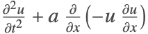
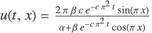
Wolfram Language code: op = D[u[t, x], t] + Inactive[Plus][Inactive[Div][{{-c}}. Inactive[Grad][u[t, x], {x}], {x}], +u[t, x] * D[u[t, x], x]]

解析解：

解のパラメータを設定する．

Wolfram Language code: params = {β -> 4, c -> 1 / 20, α -> 5}

解析解を設定する．

Wolfram Language code: ares = Function[{t, x}, Evaluate[(2 π β c Exp[-c π ^ 2t]Sin[π x]) / (α + β Exp[-c π ^ 2t]Cos[π x]) /. params]]

境界条件：

境界条件は解析解から推測される．

および

境界条件を設定する．

Wolfram Language code: bcs = {DirichletCondition[u[t, x] == 0, True]}

初期条件：

初期条件は解析解から推測される．

初期条件を設定する．

Wolfram Language code: ics = {u[0, x] == ares[0, x]}

領域：

領域を設定する．

Wolfram Language code: region = Line[{{0}, {1}}]

テスト1：

非アクティブな形式の偏微分方程式をテストする．

Wolfram Language code:

VerificationTest[
	nlfun = NDSolveValue[{op == 0, bcs, ics} /. params, u, {t, 0, 2}, Element[{x}, region], Method -> topts];
	Norm[Table[nlfun[t, x] - ares[t, x], {t, 0, 1, 0.1}, {x, 0, 1, 0.1}]] < 10 ^ -3, 
	True, 
	TestID -> "FEM-NL-Transient-1D-Single-Convection-0002-A"
	]

テスト2：

偏微分方程式をテストする．

Wolfram Language code:

VerificationTest[
	aeqn = Activate[{op == 0, bcs, ics} /. params];
	anlfun = NDSolveValue[aeqn, u, {t, 0, 1}, Element[{x}, region], Method -> topts];
	Norm[Table[anlfun[t, x] - ares[t, x], {t, 0, 1, 0.1}, {x, 0, 1, 0.1}]] < 10 ^ -3, 
	True, 
	TestID -> "FEM-NL-Transient-1D-Single-Convection-0002-B"
	]

反応—FEM-NL-Transient-1D-Single-Reaction-0001

テストの参考文献：

[3], Exact Solutions > Nonlinear Partial Differential Equations >Second-Order Parabolic Partial Differential Equations > Fisher Equation; Equation 1.1.1; Fisher equation.

方程式：

非アクティブな形式で方程式を設定する．

Wolfram Language code:

op = D[u[t, x], t] + Inactive[Plus][Inactive[Div][{{-1}}. Inactive[Grad][u[t, x], {x}], {x}], -a * u[t, x] * (1 - u[t, x])]

解析解：

解のパラメータを設定する．

Wolfram Language code: params = {C -> 1, a -> 2 / 3}

解析解を設定する．

Wolfram Language code: ares = Function[{t, x}, Evaluate[1 / (1 + C Exp[-5 / 6 a t - 1 / 6 Sqrt[6 a]x]) ^ 2 /. params]]

境界条件：

境界条件は指定されない．境界条件は解析解から推測される．

および

境界条件を設定する．

Wolfram Language code: bcs = {DirichletCondition[u[t, x] == ares[t, 0], x == 0], DirichletCondition[u[t, x] == ares[t, 1], x == 1]}

初期条件：

初期条件は指定されない．初期条件は解析解から推測される．

初期条件を設定する．

Wolfram Language code: ics = {u[0, x] == ares[0, x]}

領域：

領域を設定する．

Wolfram Language code: region = Line[{{0}, {1}}]

テスト1：

非アクティブな形式の偏微分方程式をテストする．

Wolfram Language code:

VerificationTest[
	nlfun = NDSolveValue[{op == 0, bcs, ics} /. params, u, {t, 0, 1}, Element[{x}, region], Method -> topts];
	Norm[Table[nlfun[t, x] - ares[t, x], {t, 0, 1, 0.1}, {x, 0, 1, 0.1}]] < 10 ^ -3, 
	True, 
	TestID -> "FEM-NL-Transient-1D-Single-Reaction-0001-A"
	]

テスト2：

偏微分方程式をテストする．

Wolfram Language code:

VerificationTest[
	aeqn = Activate[{op == 0, bcs, ics} /. params];
	anlfun = NDSolveValue[aeqn, u, {t, 0, 1}, Element[{x}, region], Method -> topts];
	Norm[Table[anlfun[t, x] - ares[t, x], {t, 0, 1, 0.1}, {x, 0, 1, 0.1}]] < 10 ^ -3, 
	True, 
	TestID -> "FEM-NL-Transient-1D-Single-Reaction-0001-B"
	]

反応—FEM-NL-Transient-1D-Single-Reaction-0002

テストの参考文献：

[3], Exact Solutions > Nonlinear Partial Differential Equations >Second-Order Hyperbolic Partial Differential Equations > Klein–Gordon Equation with a Power-Law Nonlinearity; Equation 2.1.1; Klein--Gordon equation with a power-law nonlinearity.

方程式：

非アクティブな形式で方程式を設定する．

Wolfram Language code:

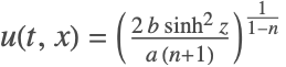
op = D[u[t, x], {t, 2}] + Inactive[Plus][Inactive[Div][{{-1}}. Inactive[Grad][u[t, x], {x}], {x}], -a * u[t, x] - b u[t, x] ^ n]

解析解：

, ,

解のパラメータを設定する．

Wolfram Language code: params = {C[1] -> -1, C[2] -> -1, a -> 1, b -> 1, n -> 2}

Wolfram Language code: a > 0 && b (n + 1) > 0 /. params

解析解を設定する．

Wolfram Language code:

ares = Function[{t, x}, Evaluate[Block[{z = 1 / 2 Sqrt[a](1 - n)(x Sinh[C[1]] + t Cosh[C[1]]) + C[2]}, ((2 b Sinh[z] ^ 2) / (a * (n + 1))) ^ (1 / (1 - n))] /. params]]

境界条件：

境界条件は指定されない．境界条件は解析解から推測される．

および

境界条件を設定する．

Wolfram Language code: bcs = {DirichletCondition[u[t, x] == ares[t, 0], x == 0], DirichletCondition[u[t, x] == ares[t, 1], x == 1]}

初期条件：

初期条件は指定されない．初期条件は解析解から推測される．

初期条件を設定する．

Wolfram Language code: ics = {u[0, x] == ares[0, x], Derivative[1, 0][u][0, x] == D[ares[t, x], t] /. t -> 0}

領域：

領域を設定する．

Wolfram Language code: region = Line[{{0}, {1}}]

テスト1：

非アクティブな形式の偏微分方程式をテストする．

Wolfram Language code:

VerificationTest[
	nlfun = NDSolveValue[{op == 0, bcs, ics} /. params, u, {t, 0, 1}, Element[{x}, region], Method -> topts];
	Norm[Table[nlfun[t, x] - ares[t, x], {t, 0, 1, 0.1}, {x, 0, 1, 0.1}]] < 10 ^ -2, 
	True, 
	TestID -> "FEM-NL-Transient-1D-Single-Reaction-0002-A"
	]

テスト2：

偏微分方程式をテストする．

Wolfram Language code:

VerificationTest[
	aeqn = Activate[{op == 0, bcs, ics} /. params];
	anlfun = NDSolveValue[aeqn, u, {t, 0, 1}, Element[{x}, region], Method -> topts];
	Norm[Table[anlfun[t, x] - ares[t, x], {t, 0, 1, 0.1}, {x, 0, 1, 0.1}]] < 10 ^ -2, 
	True, 
	TestID -> "FEM-NL-Transient-1D-Single-Reaction-0002-B"
	]

負荷—FEM-NL-Transient-1D-Single-Load-0001

テストの参考文献：

[3], Exact Solutions > Nonlinear Partial Differential Equations >Second-Order Parabolic Partial Differential Equations > Equation 1.1.5;

方程式：

非アクティブな形式で方程式を設定する．

Wolfram Language code: op = D[u[t, x], t] + Inactive[Plus][Inactive[Div][{{-1}}. Inactive[Grad][u[t, x], {x}], {x}], -a, -b Exp[λ u[t, x]]]

解析解：

解のパラメータを設定する．

Wolfram Language code: params = {C -> -1, a -> 1, b -> -2, λ -> 3 / 2}

解析解を設定する．

Wolfram Language code: ares = Function[{t, x}, Evaluate[-2 / λ Log[Sqrt[-b / a] + C Exp[-Sqrt[a λ / 2]x - 1 / 2a λ t]] /. params]]

境界条件：

境界条件は指定されない．境界条件は解析解から推測される．

および

境界条件を設定する．

Wolfram Language code: bcs = {DirichletCondition[u[t, x] == ares[t, 0], x == 0], DirichletCondition[u[t, x] == ares[t, 1], x == 1]}

初期条件：

初期条件は指定されない．初期条件は解析解から推測される．

初期条件を設定する．

Wolfram Language code: ics = {u[0, x] == ares[0, x]}

領域：

領域を設定する．

Wolfram Language code: region = Line[{{0}, {1}}]

テスト1：

非アクティブな形式の偏微分方程式をテストする．

Wolfram Language code:

VerificationTest[
	nlfun = NDSolveValue[{op == 0, bcs, ics} /. params, u, {t, 0, 1}, Element[{x}, region], Method -> topts];
	Norm[Table[nlfun[t, x] - ares[t, x], {t, 0, 1, 0.1}, {x, 0, 1, 0.1}]] < 10 ^ -3, 
	True, 
	TestID -> "FEM-NL-Transient-1D-Single-Load-0001-A"
	]

テスト2：

偏微分方程式をテストする．

Wolfram Language code:

VerificationTest[
	aeqn = Activate[{op == 0, bcs, ics} /. params];
	anlfun = NDSolveValue[aeqn, u, {t, 0, 1}, Element[{x}, region], Method -> topts];
	Norm[Table[anlfun[t, x] - ares[t, x], {t, 0, 1}, {x, 0, 1, 0.1}]] < 10 ^ -3, 
	True, 
	TestID -> "FEM-NL-Transient-1D-Single-Load-0001-B"
	]

負荷—FEM-NL-Transient-1D-Single-Load-0002

テストの参考文献：

[3], Exact Solutions > Nonlinear Partial Differential Equations >Second-Order Hyperbolic Partial Differential Equations > Modified Liouville Equation; Equation 2.1.3;

方程式：

非アクティブな形式で方程式を設定する．

Wolfram Language code:

op = D[u[t, x], {t, 2}] + Inactive[Plus][a ^ 2 Inactive[Div][{{-1}}. Inactive[Grad][u[t, x], {x}], {x}], -b Exp[β u[t, x]]]

解析解：

解のパラメータを設定する．

Wolfram Language code: params = {A -> 1, B -> 2, C -> 1, a -> 1, b -> 1, β -> 3 / 2}

解析解を設定する．

Wolfram Language code: ares = Function[{t, x}, Evaluate[1 / β Log[2(B ^ 2 - a ^ 2A ^ 2) / (b β (A x + B t + C) ^ 2)] /. params]]

境界条件：

境界条件は指定されない．境界条件は解析解から推測される．

および

境界条件を設定する．

Wolfram Language code: bcs = {DirichletCondition[u[t, x] == ares[t, 0], x == 0], DirichletCondition[u[t, x] == ares[t, 1], x == 1]}

初期条件：

初期条件は指定されない．初期条件は解析解から推測される．

初期条件を設定する．

Wolfram Language code: ics = {u[0, x] == ares[0, x], Derivative[1, 0][u][0, x] == D[ares[t, x], t] /. t -> 0}

領域：

領域を設定する．

Wolfram Language code: region = Line[{{0}, {1}}]

テスト1：

Wolfram Language code:

VerificationTest[
	nlfun = NDSolveValue[{op == 0, bcs, ics} /. params, u, {t, 0, 1}, Element[{x}, region], Method -> topts];
	Norm[Table[nlfun[t, x] - ares[t, x], {t, 0, 1, 0.1}, {x, 0, 1, 0.1}]] < 10 ^ -2, 
	True, 
	TestID -> "FEM-NL-Transient-1D-Single-Load-0002-A"
	]

テスト2：

偏微分方程式をテストする．

Wolfram Language code:

VerificationTest[
	aeqn = Activate[{op == 0, bcs, ics} /. params];
	anlfun = NDSolveValue[aeqn, u, {t, 0, 1}, Element[{x}, region], Method -> topts];
	Norm[Table[anlfun[t, x] - ares[t, x], {t, 0, 1, 0.1}, {x, 0, 1, 0.1}]] < 10 ^ -2, 
	True, 
	TestID -> "FEM-NL-Transient-1D-Single-Load-0002-B"
	]

テスト3：

時間ステップサイズの極限を低くする．

Wolfram Language code:

VerificationTest[
	nlfun = NDSolveValue[{op == 0, bcs, ics} /. params, u, {t, 0, 1}, Element[{x}, region], Method -> topts, "MaxStepSize" -> Max[Abs[Subtract@@@Partition[anlfun["Coordinates"][[1]], 2, 1]]]];
	Norm[Table[nlfun[t, x] - ares[t, x], {t, 0, 1, 0.1}, {x, 0, 1, 0.1}]] < 10 ^ -2, 
	True, 
	TestID -> "FEM-NL-Transient-1D-Single-Load-0002-C"
	]

非アクティブな偏微分方程式を再度定式化する．

Wolfram Language code:

VerificationTest[
	nlfun = NDSolveValue[{D[u[t, x], {t, 2}] + Plus[a ^ 2 Inactive[Div][{{-1}}. Inactive[Grad][u[t, x], {x}], {x}], -b Exp[β u[t, x]]] == 0, bcs, ics} /. params, u, {t, 0, 1}, Element[{x}, region], Method -> topts];
	Norm[Table[nlfun[t, x] - ares[t, x], {t, 0, 1, 0.1}, {x, 0, 1, 0.1}]] < 10 ^ -2, 
	True, 
	TestID -> "FEM-NL-Transient-1D-Single-Load-0002-D"
	]

反応-拡散—FEM-NL-Transient-1D-Single-Reaction-Diffusion-0001

テストの参考文献：

[3], Exact Solutions > Nonlinear Partial Differential Equations >Second-Order Parabolic Partial Differential Equations > Fisher Equation; Equation 1.2.5;

方程式：

非アクティブな形式で方程式を設定する．

Wolfram Language code:

op = D[u[t, x], t] + Inactive[Plus][a Inactive[Div][{{-u[t, x] ^ (2 n)}}. Inactive[Grad][u[t, x], {x}], {x}], -b * u[t, x] ^ (1 - n)]

解析解：

解のパラメータを設定する．

Wolfram Language code: params = {C[1] -> 0, C[2] -> 5, a -> 1, b -> 0, n -> 1}

解析解を設定する．

Wolfram Language code:

ares = Function[{t, x}, Evaluate[With[{k = 2a(n + 1) / n}, ((x + C[1]) / Sqrt[C[2] - k t] - (b n ^ 2) / (3 a (n + 1))(C[2] - k t)) ^ (1 / n)] /. params]]

境界条件：

境界条件は指定されない．境界条件は解析解から推測される．

および

境界条件を設定する．

Wolfram Language code: bcs = {DirichletCondition[u[t, x] == ares[t, x], True]}

初期条件：

初期条件は指定されない．初期条件は解析解から推測される．

初期条件を設定する．

Wolfram Language code: ics = {u[0, x] == ares[0, x]}

領域：

領域を設定する．

Wolfram Language code: region = Line[{{1}, {2}}]

テスト1：

非アクティブな形式の偏微分方程式をテストする．

Wolfram Language code:

VerificationTest[
	nlfun = NDSolveValue[{op == 0, bcs, ics} /. params, u, {t, 0, 1}, Element[{x}, region], Method -> topts];
	Norm[Table[nlfun[t, x] - ares[t, x], {t, 0, 0.1, 0.01}, {x, 1, 2, 0.1}]] < 10 ^ -3, 
	True, 
	TestID -> "FEM-NL-Transient-1D-Single-Reaction-Diffusion-0001-A"
	]

テスト2：

アクティベートされた偏微分方程式をテストする．

Wolfram Language code:

VerificationTest[
	aeqn = Activate[{op == 0, bcs, ics} /. params];
	anlfun = NDSolveValue[Activate[{op == 0, bcs, ics}] /. params, u, {t, 0, 1}, Element[{x}, region], Method -> topts];
	Norm[Table[anlfun[t, x] - ares[t, x], {t, 0, 0.1, 0.01}, {x, 1, 2, 0.1}]] < 10 ^ -3, 
	True, 
	TestID -> "FEM-NL-Transient-1D-Single-Reaction-Diffusion-0001-B"
	]

二次元の単一方程式

このセクションには，単一方程式を含む時間依存の非線形偏微分方程式の例が含まれる．

拡散—FEM-NL-Stationary-2D-Single-Diffusion-0001

テストの参考文献：

[5], Example 6.3.6, page 100

方程式：

非アクティブな形式で方程式を設定する．

Wolfram Language code:

op = 175 D[u[t, x, y], t] + Inactive[Div][-{{k[u[t, x, y]], 0}, {0, k[u[t, x, y]]}}. Inactive[Grad][u[t, x, y], {x, y}], {x, y}] /. k :> Function[u, 1 / 200 u + 1];

解析解：

なし

人工的な解

解析解を設定する．

Wolfram Language code: ares = Function[{t, x, y}, 68(1 + Cos[π x / 2])(1 + Cos[π y / 2])Exp[-t]]

人工的な解の右辺を構築する．

Wolfram Language code: f = Activate[op /. u -> ares]

境界条件：

境界条件を設定する．

Wolfram Language code: bcs = {DirichletCondition[u[t, x, y] == 0, True]}

初期条件：

初期条件は指定されない．初期条件は解析解から推測される．

初期条件を設定する．

Wolfram Language code: ics = {u[0, x, y] == ares[0, x, y]}

領域：

領域を設定する．

Wolfram Language code: region = Rectangle[{-2, -2}, {2, 2}]

テスト1：

非アクティブな形式の偏微分方程式をテストする．

Wolfram Language code:

VerificationTest[
	nlfun = NDSolveValue[{op == f, bcs, ics}, u, {t, 0, 1}, Element[{x, y}, region], MaxStepSize -> 0.01];
	Norm[Table[nlfun[1, x, y] - ares[1, x, y], {x, -2, 2, 0.1}, {y, -2, 2, 0.1}]] < 10 ^ -1, 
	True, 
	TestID -> "FEM-NL-Transient-2D-Single-Diffusion-0001-A"
	]

メッシュの最大セルの大きさを小さくし，最大ステップサイズをより小さくすることによって，より高品質の結果が得られる．ここでそうしなかったのは，テストにより長い時間かかるからである．

テスト結果の調査

このセクションには，実行したテストの評価が含まれる．TestResultObjectのすべてのインスタンスを集め，TestReportを生成する．

ノートブックからTestResultObjectを抽出し，TestReportを生成する．

Wolfram Language code:

nb = EvaluationNotebook[];
cso = Cells[nb, CellStyle -> {"Output"}];
tros = Cases[ToExpression[First[NotebookRead[#]]]& /@ cso, _TestResultObject];
report = TestReport[tros]

実行に失敗したテストを調べる．

Wolfram Language code: Column /@ (Normal /@ report["TestsFailed"])//TabView

上の表が空であれば，すべてのテストが成功したということである．

参考文献

[1] Advanced Topics in Finite Element Analysis of Structures; Bhatti, M. Asghar; Wiley; ISBN: 978-81-265-4537-7.

[2] Nonlinear Finite Element Analysis; Reddy, J. N.; Oxford; ISBN: 978-0-19-852529-5.

[3] "EqWorld, The World of Mathematical Equations"; http://eqworld.ipmnet.ru.

[4] Automated Solution of Differential Equations by the Finite Element Method; Logg, A; Mardal, K-A; Wells, G. N.; Springer; ISBN: 978-3-642-23098-1.

[5] "Nonlinear, Transient Conduction Heat Transfer Using a Discontinuous Galerkin Hierarchical Finite Element Method"; Sanders, J. C.; http://www.phys.uconn.edu/~sanders/ThesisMain.pdf.

Top