Electrostatically Actuated MEMS Device
Introduction
In this application example, a micro-electromechanical system (MEMS) device is modeled. MEMS devices are widely used, for example, switches in sensors and actuators [Sumant et al., 2009]. The MEMS device modeled consists of a thin movable beam, an electrode suspended over a fixed electrode.
Suppose a voltage difference is applied between the fixed and the movable electrodes. In that case, the movable electrode will have a deformation caused by the induced surface charges. This deformation can be used for actuation or sensing functions. The relation between the deformation and the potential difference makes this device a coupled electro-mechanical system.
A traditional method to solve this model is by performing a series of electrostatic and mechanical analyses where, in each step, a new mesh of the deformed beam will be needed. The simulation is then alternating between the mechanical and electrostatic and mesh update until the deformation reaches a state of equilibrium. This is quite an involved approach.
This application example makes use of a simpler approach proposed by [Sumant et al., 2009]. With this approach, the electrostatic analysis is done only once, and then the mechanical analysis is performed in a second step. This avoids the re-creation of a mesh in each step, and this method speeds up the simulation process.
The authors [Sumant et al., 2009] achieved both a good quality simulation and a speedy result by making a crucial simplification: The surface charge density on the movable electrode in the deformed geometry was approximated in terms of the surface charge density in the non-deformed geometry and displacements of the movable electrode. This allows one to dispense with the remeshing.
The device to be modeled and illustrated below is a cantilever series switch, one of the most important radio frequency (RF) MEMS switches. The switch consists of a beam suspended over a bottom ground electrode, part of a microwave planar transmission line. The bottom ground electrode is on top of a silicon substrate [Sumant et al., 2009].
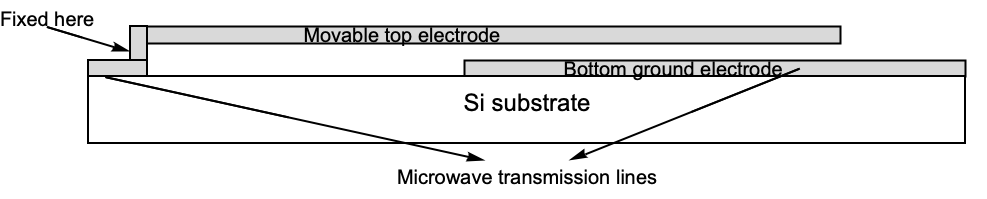
Geometry and components of a cantilever series switch.
A voltage difference must be applied between the electrodes to make the switch work. This voltage difference and the electric field produced induce surface charge densities on the surfaces of the electrodes. These surface charges give rise to electrostatic forces between both electrodes. Since the bottom electrode is fixed, the forces will only deform the top electrode. This new deformation changes the distribution of surface charges, and consequently, the new resultant forces bend the beam further. This process is counter acted by the stiffness of the beam and continues until a state of equilibrium is reached.
In the following sections, the method to solve for the deformation of the movable electrode of the switch will be explained in detail [Sumant et al., 2009].
Needs["NDSolve`FEM`"]Multiphysics
Two physical domains are involved in this application: the electrostatic model and the structural mechanics model. The coupling between the two models is one way: the electrode deformation depends only on the electrostatic pressure.
The electrostatic pressure ![]() [
[![]() ] is given by the following equation:
] is given by the following equation:
where ![]() is the absolute electric permittivity in units of [
is the absolute electric permittivity in units of [![]() ] and
] and ![]() is the surface charge density in units of [
is the surface charge density in units of [![]() ]. The surface charge density is given by:
]. The surface charge density is given by:
where ![]() is the boundary unit normal and
is the boundary unit normal and ![]() is the gradient of the electric potential
is the gradient of the electric potential ![]() [
[![]() ].
].
Using the fact that the electric field intensity is given by ![]() [
[![]() ] and using the linear constitutive relation
] and using the linear constitutive relation ![]() , the surface charge density can be rewritten in terms of the electric flux density
, the surface charge density can be rewritten in terms of the electric flux density ![]() [
[![]() ]:
]:
where ![]() is the normal component of the electric flux density.
is the normal component of the electric flux density.
Eq.1 restates the fact that at a conductor surface the electric field ![]() and the electric flux density
and the electric flux density ![]() have only a normal component. Thus, the electrostatic pressure can be also expressed in terms of the normal component of the electric flux density:
have only a normal component. Thus, the electrostatic pressure can be also expressed in terms of the normal component of the electric flux density:
To calculate the normal component of the electric flux density ![]() the magnitude of the electric flux density
the magnitude of the electric flux density ![]() is used:
is used:
As there are no tangential components on the conductor surface, the magnitude can be expressed as follows:
So the electrostatic pressure can be rewritten in terms of the electric flux density magnitude ![]() :
:
The proposed method mentioned in [Sumant et al., 2009] is based on the fact that the electric flux density on the movable electrode in the deformed electrode can be approximated in terms of the electric flux density on the non-deformed electrode and the updated displacement of the movable electrode.
Then, the expression that relates the charge density in the deformed geometry ![]() to the charge density on the movable electrode in the non-deformed geometry
to the charge density on the movable electrode in the non-deformed geometry ![]() is the following:
is the following:
where ![]() [
[![]() ] is the distance or gap between the movable and fixed electrodes in the absence of actuation, and
] is the distance or gap between the movable and fixed electrodes in the absence of actuation, and ![]() [
[![]() ] is the displacement of the movable electrode in the
] is the displacement of the movable electrode in the ![]() direction at position
direction at position ![]() along its axis.
along its axis.
Eq. 2 works well for MEMS devices involving cantilevers or supported beams with homogeneous dielectrics and for devices with electrodes of comparable lengths, as is in this case. Details about the derivation of Eq. 3 is found in [Sumant et al., 2009].
The following procedure is followed to perform the electro-mechanical analysis using Eq. 4:
1. First, the electrostatic model is solved in the non-deformed geometry.
2. Then, the load boundary conditions for the mechanical model are computed using the calculated charge density values along the movable electrode and computing the pressure ![]() using Eq. 5.
using Eq. 5.
3. Next, the structural mechanics model is constructed, and the deformation of the movable electrode is computed.
4. Then, the calculated deformation in the ![]() direction of the movable electrode is used to update the electric flux density along the boundary of the movable electrode using Eq. 6.
direction of the movable electrode is used to update the electric flux density along the boundary of the movable electrode using Eq. 6.
5. Finally, one must repeat steps 2 to 4 until convergence is reached. At each step, the deformation of the movable electrode is changing.
Electrostatic Analysis
In the following section, the electrostatic model will be solved using the linear electrostatic equation to get the potential distribution ![]() [
[![]() ] of the model:
] of the model:
In this model, the volume charge density ![]() is set to zero.
is set to zero.
Electrostatic Domain
The cantilever series switch is simplified by modelling the following geometry in which the silicon substrate is not included.

Domain and dimensions of the simplified cantilever series switch.
The movable top electrode is 150 [![]() ] in length and 2 [
] in length and 2 [![]() ] in thickness. The bottom electrode is 50 [
] in thickness. The bottom electrode is 50 [![]() ] in length and 2 [
] in length and 2 [![]() ] in thickness, and the bottom electrode is located 100 [
] in thickness, and the bottom electrode is located 100 [![]() ] from where the top electrode is fixed. The gap between the electrodes is 2 [
] from where the top electrode is fixed. The gap between the electrodes is 2 [![]() ].
].
The surrounding area will have a length of 350 [![]() ] and a height of 30 [
] and a height of 30 [![]() ].
].
The specification of the boundary conditions will be through boundary markers and point markers, assigned manually. To makes use of our own markers, the boundary mesh is created manually, using ToBoundaryMesh. Markers and their use in meshes are explained in detail in the section Element Marker in the Element Mesh Generation tutorial.
The coordinates used to specify the domain will be defined on the basis that the center of the rectangle of the surrounding area is at the origin ![]() .
.
scale = 10 ^ -6;c1 = {{-175, -17}, {175, -17}, {175, 13}, {-175, 13}} * scale;c2 = {{25, -2}, {75, -2}, {75, 0}, {25, 0}} * scale;c3 = {{-75, 2}, {75, 2}, {75, 4}, {-75, 4}} * scale;This geometry setup was used to match the results with the ones shown in [Sumant et al., 2009].
The boundaries of the surrounding box, the movable electrode and the fixed electrodes will have the markers ![]() , respectively.
, respectively.
bmarkers = {1, 1, 1, 1, 2, 2, 2, 2, 3, 3, 3, 3};bmesh = ToBoundaryMesh["Coordinates" -> Join[c1, c2, c3], "BoundaryElements" -> {LineElement[{{1, 2}, {2, 3}, {3, 4}, {4, 1}, {5, 6}, {6, 7}, {7, 8}, {8, 5}, {9, 10}, {10, 11}, {11, 12}, {12, 9}}, bmarkers]}];When simulating an electrostatic model, every metal or electrode inside the domain needs to be removed. This is possible because metals in the electrostatic regime have the same potential everywhere and can thus be treated as boundaries rather than volume regions.
mesh = ToElementMesh[bmesh, "RegionHoles" -> {{0, 3}, {40, -1}} * scale, MaxCellMeasure -> {"Length" -> 5 * scale}];A max cell measure value was applied to the mesh to get a more accurate result.
Electrostatic Parameters Setup
In a next step, the material parameters and the electrostatic equation are set up. The only material parameter that needs to be defined is the unitless relative permittivity ![]() [
[![]() ] of the surrounding area. In [Sumant et al., 2009] there is no specification of the material, but as there is no volume charge density, the choice of the relative permittivity will not affect the solution as long as the value is a constant.
] of the surrounding area. In [Sumant et al., 2009] there is no specification of the material, but as there is no volume charge density, the choice of the relative permittivity will not affect the solution as long as the value is a constant.
vars = {V[x, y], {x, y}};
pars = <|"RelativePermittivity" -> 1|>;op = ElectrostaticPDEComponent[vars, pars];Boundary Conditions
The way the switch works is by applying a voltage difference between the electrodes. A potential of ![]() is applied to the boundaries of the movable electrode, and the boundaries of the fixed electrode are set to ground
is applied to the boundaries of the movable electrode, and the boundaries of the fixed electrode are set to ground ![]() . The exterior boundaries also will be set to
. The exterior boundaries also will be set to ![]() .
.
These conditions can be specified with ElectricPotentialCondition. ElectricPotentialCondition works as a DirichletCondition, so the markers that are used to specify these boundary conditions are point markers. The markers specified when building the boundary mesh were boundary elements, and the point markers will inherit their values from the boundary markers.
Legended[bmesh["Wireframe"["MeshElementStyle" -> {Blue, Green, Red}, ImageSize -> Medium]], SwatchLegend[...]]mesh["PointElementMarkerUnion"]Legended[mesh["Wireframe"["MeshElement" -> "PointElements", "MeshElementStyle" -> {Blue, Green, Red}, ImageSize -> Medium]], SwatchLegend[...]]The markers ![]() will be used to specify the ground potential, and the marker
will be used to specify the ground potential, and the marker ![]() for the potential at the movable electrode.
for the potential at the movable electrode.
Subscript[Γ, ground] = ElectricPotentialCondition[ElementMarker == 1 || ElementMarker == 2, vars, pars, <|"ElectricPotential" -> 0|>];Subscript[Γ, p] = ElectricPotentialCondition[ElementMarker == 3, vars, pars, <|"ElectricPotential" -> 20|>];Solution and Visualization
Now that the setup of the whole electrostatic PDE model is complete, the model can be solved.
electricPotentialFun = NDSolveValue[{op == 0, Subscript[Γ, p], Subscript[Γ, ground]}, V, {x, y}∈mesh];DensityPlot[electricPotentialFun[x, y], {x, y}∈mesh, ...]From this solution, the magnitude of the electric flux density ![]() will be computed according to the following equation:
will be computed according to the following equation:
where the absolute permittivity ![]() is the vacuum permittivity
is the vacuum permittivity ![]() times the relative permittivity
times the relative permittivity ![]() .
.
Efield = -Grad[electricPotentialFun[x, y], {x, y}];absEfield = Sqrt[Efield[[1]] ^ 2 + Efield[[2]] ^ 2];eps0 = PDEModels`DefaultModelParameters[vars, pars, "Electrostatics"]["VacuumPermittivity"];absD0field = eps0 * absEfield;Structural Mechanics Analysis
Steps 2 to 5, mentioned in the Multiphysics section will be performed in this section.
1. Define load boundary conditions for the mechanical model.
2. Compute the deformation of the movable electrode.
3. Update the electric flux density along the boundary of the movable electrode.
4. Repeat steps 2 to 4 until convergence is reached.
All these steps involve a plane stress structural mechanics model. In structural mechanics, the plane stress relation, Eq. 7, describes the deformation of thin objects. Here, "thin" means thin relative to the other dimensions of the object. The two dependent variables ![]() ,
, ![]() denote the deformation in the
denote the deformation in the ![]() and
and ![]() directions, respectively. As material data, Young's modulus
directions, respectively. As material data, Young's modulus ![]() [
[![]() ] and the Poisson ratio
] and the Poisson ratio ![]() [
[![]() ] need to be specified.
] need to be specified.
The equilibrium equation, Eq. 8, which denotes the force balance in the ![]() and
and ![]() directions, is then used as the governing PDE of the structural mechanics model. On the right-hand side,
directions, is then used as the governing PDE of the structural mechanics model. On the right-hand side, ![]() and
and ![]() model any external pressure that may act on the object.
model any external pressure that may act on the object.
In this model, the electrostatic pressure is the only external force that applies on the movable electrode beam and is coupled to the plane-stress PDE, Eq. 9, as the source term on the right-hand side.
Domain
The structural mechanics analysis will be performed only on the movable electrode, since it is the only structure in the system that will undergo deformation. This mesh will also be built manually and boundary conditions will be specified with element markers.
bmeshSM = ToBoundaryMesh["Coordinates" -> c3, "BoundaryElements" -> {LineElement[{{1, 2}, {2, 3}, {3, 4}, {4, 1}}]}];bmeshSM["Wireframe"[ImageSize -> Medium]]meshSM = ToElementMesh[bmeshSM, MaxCellMeasure -> {"Length" -> 1 * scale}];Structural Mechanics Parameters Setup
First, the variables for the solid mechanics part of the model are defined.
varsSM = {{u[x, y], v[x, y]}, {x, y}};The device is modeled as a plane stress case.
pars["SolidMechanicsModelForm"] = "PlaneStress";The mechanical properties of the movable electrode are given by its Young modulus ![]() [
[![]() ] and its Poisson ratio
] and its Poisson ratio ![]() [
[![]() ].
].
pars["YoungModulus"] = 170*^9;
pars["PoissonRatio"] = 0.34;
This model uses a plane stress formulation, and a thickness of ![]() [
[![]() ] is assumed.
] is assumed.
pars["Thickness"] = 1 * scale;opSM = SolidMechanicsPDEComponent[varsSM, pars];Boundary Conditions
Next, boundary conditions to which the movable electrode is subjected to need to be defined. The first boundary at the movable electrode is a fixed condition at the left side implemented with SolidFixedCondition. This fixed condition makes use of point markers to know where to apply the condition.
meshSM["PointElementMarkerUnion"]meshSM["Wireframe"["MeshElement" -> "PointElements", "MeshElementMarkerStyle" -> Black, "MeshElementStyle" -> {Blue, Brown, Green, Red, Darker[Green], Orange, Purple, Gray}, PlotRange -> {{-78, -70}, {1.5, 4.5}} * scale]]The markers needed to specify the SolidFixedCondition are the numbers ![]() .
.
Subscript[Γ, wall] = SolidFixedCondition[ElementMarker == 4 || ElementMarker == 6 || ElementMarker == 8, varsSM, pars];The second boundary condition to apply is a SolidBoundaryLoadValue. This boundary will specify the pressure that the electrode will feel due to the induced surface charge densities. The pressure will be exerted at all boundaries of the electrode except the fixed left side. A helper function electrostaticPressure will compute the pressure following equations 10 and 11.
Legended[bmeshSM["Wireframe"["MeshElementMarkerStyle" -> Black, "MeshElementStyle" -> {Blue, Brown, Green, Red}, AspectRatio -> 1 / 10]], SwatchLegend[...]]The boundary with marker 4 is the fixed end. Markers ![]() are associated with the pressure boundary condition.
are associated with the pressure boundary condition.
Electrostatic pressure
In this section, the function for the electrostaticPressure is defined based on the details given in the multiphysics section. The electrostatic pressure ![]() [
[![]() ] is given by the following formula:
] is given by the following formula:
where ![]() is the absolute electric permittivity and
is the absolute electric permittivity and ![]() the electric flux density.
the electric flux density.
After the first displacement of the movable electrode is computed, the electric flux density along the movable electrode is updated using the calculated displacement in the ![]() direction
direction ![]() with the following equation:
with the following equation:
where ![]() [
[![]() ] is the distance or gap between the movable and fixed electrodes in the absence of actuation, and
] is the distance or gap between the movable and fixed electrodes in the absence of actuation, and ![]() [
[![]() ] is the displacement of the movable electrode in the
] is the displacement of the movable electrode in the ![]() direction at position
direction at position ![]() along its axis.
along its axis.
When the function is used in the first displacement computation, the movable electrode is undeformed ![]() , leading to
, leading to ![]() .
.
electrostaticPressure[{x_, y_}, eps0_, absD0field_, vdisplacement_]  :=
 Module[{absDfield, G, ePressure},
	G = 2*^-6;
	absDfield = (absD0field * G) / (G - Abs[vdisplacement]);
	ePressure = (absDfield ^ 2) / (2 * eps0)
  ]
The SolidBoundaryLoadValue specified here will be a function of the displacement in the ![]() direction,
direction, ![]() . The first iteration of the solid mechanics analysis will use a load boundary condition with a zero displacement, and for the next iterations the previous deformations are taken into account.
. The first iteration of the solid mechanics analysis will use a load boundary condition with a zero displacement, and for the next iterations the previous deformations are taken into account.
boundaryLoad[vdisplacement_] := SolidBoundaryLoadValue[ElementMarker != 4, varsSM, pars, <|"Pressure" -> {Indexed[BoundaryUnitNormal[x, y], 1], Indexed[BoundaryUnitNormal[x, y], 2]} * electrostaticPressure[{x, y}, eps0, absD0field, vdisplacement]|>];Solution
It is convenient to define a pseudo parametric function that will solve the mechanical PDE, based on different displacements inputs.
paramFun[vdisplacement_] := NDSolveValue[{opSM == boundaryLoad[vdisplacement], Subscript[Γ, wall]}, {u[x, y], v[x, y]}, {x, y}∈meshSM]One might think to use ParametricNDSolve for this parametric setup; however, in this version of the Wolfram Language, ParametricFunction does not support the input of InterpolatingFunction objects as a parametric argument. Defining the pseudo parametric function paramFun is a simple way around that.
The idea is now to solve the mechanical system with an initial 0 displacement and use the ![]() direction component of the solution for the next iteration.
direction component of the solution for the next iteration.
{uFun, vFun} = paramFun[Function[0][x, y]];To check for convergence, the maximum displacement in the ![]() direction of the movable electrode is monitored. The system has reached its state of equilibrium if the maximum displacement value from the previous two iterations no longer changes. For this, the relative error is computed from the last two maximum displacements. Previous values are not available; they are set to zero.
direction of the movable electrode is monitored. The system has reached its state of equilibrium if the maximum displacement value from the previous two iterations no longer changes. For this, the relative error is computed from the last two maximum displacements. Previous values are not available; they are set to zero.
olddisp = 0;maxdisp = Max[Abs[vFun[[0]]["ValuesOnGrid"]]]Now, the electrostatic pressure is updated and the model solved until the electrode deformation values converge with an accuracy of ![]() .
.
AbsoluteTiming[
	While[Abs[(maxdisp - olddisp) / maxdisp] > 1*^-9,
	{uFun, vFun} = paramFun[vFun];
	olddisp = maxdisp;
	maxdisp = Max[Abs[vFun[[0]]["ValuesOnGrid"]]];
	]]
The final maximum displacement of the tip of the cantilever beam matches the value shown in Figure 5(b) of [Sumant et al., 2009].
maxdispVisualization and Post-processing
What remains is to compute the von Mises stress of the deformed movable electrode and visualize it.
deformedMesh = ElementMeshDeformation[meshSM, {uFun, vFun}, "ScalingFactor" -> 1];In order to plot the deformation to scale "ScalingFactor" is set to 1.
strain = SolidMechanicsStrain[varsSM, pars, {uFun, vFun}];stress = SolidMechanicsStress[varsSM, pars, strain];vonMisesStress = VonMisesStress[varsSM, pars, stress];deformedvonMisesStress = ElementMeshInterpolation[deformedMesh, vonMisesStress[[0]]["ValuesOnGrid"]];DensityPlot[deformedvonMisesStress[x, y], {x, y}∈deformedMesh, ...]The fixed condition and the electrostatic forces exerted on the top electrode caused this bending of the electrode. From this plot, one can deduce that the electrostatic forces are attractive.
Show[DensityPlot[deformedvonMisesStress[x, y], {x, y}∈deformedMesh, PlotRange -> All, AspectRatio -> 1 / 2], ...]To increase the displacement of the movable electrode, one can make bigger the voltage difference between both electrodes.
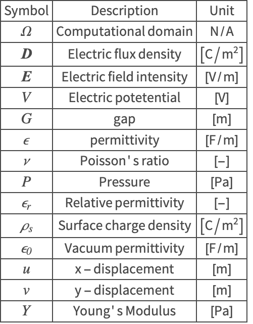
Nomenclature
References
1. Sumant, P. S., Aluru, N. R. and Cangellaris, A. C. (2009). "A Methodology for Fast Finite Element Modeling of Electrostatically Actuated MEMS," International Journal for Numerical Methods in Engineering, 77(13), pp. 1789–1808.