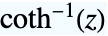
ArcCoth

ArcCoth[z]

複素数の逆双曲線余接を与える．

詳細

記号操作・数値操作の両方に適した数学関数である．
特別な引数の場合，ArcCothは自動的に厳密値を計算する．
ArcCothは任意の数値精度で評価できる．
ArcCothは自動的にリストに関数の並列的な適用を行う．
ArcCoth[z]は，複素平面上，〜の範囲で不連続な分枝切断線を持つ．
ArcCothはIntervalオブジェクトおよびCenteredIntervalオブジェクトに使うことができる． »

予備知識

ArcCothは，逆双曲線余接関数である．ArcCoth[x]は，実数について，となるようなの双曲線角度を表す．
ArcCothは自動的にリストに縫い込まれる．特別な引数の場合，ArcCothは自動的に厳密値を計算する．厳密な数式が引数として与えられると，ArcCothは任意の数値精度に評価できることがある．ArcCothを含む記号式の操作に便利なその他の演算には，FunctionExpand，TrigToExp，TrigExpand，Simplify，FullSimplifyがある．
ArcCothは，複素引数について，によって定義される．ArcCoth[z]は複素平面上で不連続な分枝切断線を持つ．
関連する数学関数には，ArcTanh，Coth，ArcCotがある．

例題

すべて開くすべて閉じる

例 (6)

数値的に評価する：

Wolfram Language code: ArcCoth[2.5]

実数の部分集合上でプロットする：

Wolfram Language code: Plot[ArcCoth[x], {x, -5, 5}]

複素数の部分集合上でプロットする：

Wolfram Language code: ComplexPlot3D[ArcCoth[z], {z, -3 - I, 3 + I}, PlotLegends -> Automatic]

原点における級数展開：

Wolfram Language code: Series[ArcCoth[x], {x, 0, 3}, Assumptions -> x > 0]

Infinityにおける漸近展開：

Wolfram Language code: Series[ArcCoth[x], {x, ∞, 5}]

特異点における漸近展開：

Wolfram Language code: Series[ArcCoth[x], {x, 1, 3}, Assumptions -> x > 1]

スコープ (43)

数値評価 (6)

数値的に評価する：

Wolfram Language code: ArcCoth[2.0]

高精度で評価する：

Wolfram Language code: N[ArcCoth[2], 50]

出力精度は入力精度に従う：

Wolfram Language code: ArcCoth[2.00000000000000000000000000000000000000000]

複素引数について評価する：

Wolfram Language code: ArcCoth[2.5 + I]

ArcCothを高精度で効率的に評価する：

Wolfram Language code: ArcCoth[2`500]//Timing

Wolfram Language code: ArcCoth[2`100000];//Timing

Intervalオブジェクトと CenteredIntervalオブジェクトを使って最悪の場合に保証される区間を計算する：

Wolfram Language code: ArcCoth[Interval[{1, Coth[5]}]]

Wolfram Language code: ArcCoth[CenteredInterval[-4, 1 / 100]]

Wolfram Language code: ArcCoth[CenteredInterval[1 - 5I, (1 + I) / 100]]

Aroundを使って平均的な場合の統計区間を計算することもできる：

Wolfram Language code: ArcCoth[Around[.9, 0.1]]

配列の要素ごとの値を計算する：

Wolfram Language code: ArcCoth[{{I, -I}, {0, -I}}]

MatrixFunctionを使って行列のArcCoth関数を計算することもできる：

Wolfram Language code: MatrixFunction[ArcCoth[#]&, {{I, -I}, {0, -I}}]

特定の値 (5)

固定点におけるArcCothの値：

Wolfram Language code: Table[ArcCoth[I n], {n, -1, 1}]

無限大における値：

Wolfram Language code: ArcCoth[Infinity]

Wolfram Language code: ArcCoth[ComplexInfinity]

ArcCothの特異点：

Wolfram Language code: ArcCoth[1]

Wolfram Language code: ArcCoth[-1]

方程式を満足させるの値を求める：

Wolfram Language code:

f[x_] := ArcCoth[x] - 1;
xzero = Solve[f[x] == 0 && 0 < x < 3, x][[1, 1]]

Wolfram Language code: Plot[f[x], {x, 0, 3}, Epilog -> Style[Point[{xzero[[2]], f[xzero[[2]]]}], PointSize[Large], Red]]

簡単な厳密値は自動的に生成される：

Wolfram Language code: ArcCoth[0]

Wolfram Language code: ArcCoth[I]

可視化 (3)

ArcCoth関数をプロットする：

Wolfram Language code: Plot[ArcCoth[x], {x, -2, 2}]

の実部をプロットする：

Wolfram Language code: ComplexContourPlot[Re[ArcCoth[z]], {z, -3 - 3 I, 3 + 3 I}, Contours -> 24]

の虚部をプロットする：

Wolfram Language code: ComplexContourPlot[Im[ArcCoth[z]], {z, -3 - 3 I, 3 + 3 I}, Contours -> 24]

の極プロット：

Wolfram Language code:

Table[PolarPlot[ArcCoth[k ϕ], {ϕ, -4π, 4π}, Sequence[Frame -> True, PlotLabel -> "k=" <> ToString[k], PlotRange -> {{-3, 3}, {-1, 3}}]], {k, 1, 4}]

関数の特性 (11)

ArcCothは，区間からの0を除くすべての実数値について定義される：

Wolfram Language code: FunctionDomain[ArcCoth[x], x]

複素領域：

Wolfram Language code: FunctionDomain[ArcCoth[z], z, Complexes]

ArcCothは0を除くすべての実数値に達する：

Wolfram Language code: FunctionRange[ArcCoth[x], x, y]

複素領域からの引数についての関数の範囲：

Wolfram Language code: FunctionRange[ArcCoth[z], z, y, Complexes]

ArcCothは奇関数である：

Wolfram Language code: ArcCoth[-x]

ArcCothは解析関数ではない：

Wolfram Language code: FunctionAnalytic[ArcCoth[x], x]

有理型でもない：

Wolfram Language code: FunctionMeromorphic[ArcCoth[x], x]

ArcCothは非減少でも非増加でもない：

Wolfram Language code: FunctionMonotonicity[ArcCoth[x], x]

ArcCothは単射である：

Wolfram Language code: FunctionInjective[ArcCoth[x], x]

Wolfram Language code: Plot[{ArcCoth[x], 1}, {x, -5, 5}]

ArcCothは全射ではない：

Wolfram Language code: FunctionSurjective[ArcCoth[x], x]

Wolfram Language code: Plot[{ArcCoth[x], 0}, {x, -2, 2}]

ArcCothは非負でも非正でもない：

Wolfram Language code: FunctionSign[ArcCoth[x], x]

[-1,1]に特異点と不連続点の両方を持つ：

Wolfram Language code: FunctionSingularities[ArcCoth[x], x]

Wolfram Language code: FunctionDiscontinuities[ArcCoth[x], x]

ArcCothは凸でも凹でもない：

Wolfram Language code: FunctionConvexity[ArcCoth[x], x]

TraditionalFormによる表示：

Wolfram Language code: ArcCoth[x]//TraditionalForm

微分 (3)

一次導関数：

Wolfram Language code: D[ArcCoth[x], x]

高次導関数：

Wolfram Language code: Table[D[ArcCoth[x], {x, n}], {n, 1, 4}]

Wolfram Language code:

Plot[Evaluate[%], {x, -1, 1}, PlotLegends -> {"First Derivative", "Second Derivative", "Third Derivative", "Fourth Derivative"}]

次導関数の式：

Wolfram Language code: D[ArcCoth[x], {x, n}]

積分 (3)

ArcCothの不定積分：

Wolfram Language code: Integrate[ArcCoth[x], x]

ArcCothを含む定積分：

Wolfram Language code: Integrate[(ArcCoth[x]/x), {x, 1, Infinity}]

その他の積分例：

Wolfram Language code: Integrate[x ArcCoth[x], x]

Wolfram Language code: Integrate[x ^ k ArcCoth[x], x]

級数展開： (4)

Seriesを使ってテイラー(Taylor)展開を求める：

Wolfram Language code: Series[ArcCoth[x], {x, 2, 4}]

の周囲のArcCothの最初の3つの近似をプロットする：

Wolfram Language code:

terms = Normal@Table[Series[ArcCoth[x], {x, 2, m}], {m, 1, 3}];
Plot[{ArcCoth[x], terms}, {x, 1, 3}, PlotRange -> {{1, 3}, {0, 3}}]

ArcCothの級数展開における一般項：

Wolfram Language code: SeriesCoefficient[ArcCoth[x], {x, 2, n}]

分岐点と分枝切断線における級数展開を求める：

Wolfram Language code: Series[ArcCoth[x], {x, 1, 1}]

Wolfram Language code: Series[ArcCoth[x], {x, (1/2), 1}]

ArcCothはベキ級数に適用できる：

Wolfram Language code: ArcCoth[SeriesData[x, 0, {1, 0, 1/3, 0, -1/45, 0, 2/945, 0, -1/4725}, -1, 8, 1]]

関数の恒等式と簡約 (3)

ArcCothを含む式を簡約する：

Wolfram Language code: Simplify[Coth[ArcCoth[x] + ArcCoth[y]] - (1 + x y/x + y)]

Logを使ってArcCothを表す：

Wolfram Language code: TrigToExp[ArcCoth[z]]

変換し直す：

Wolfram Language code: ExpToTrig[%]//FullSimplify

実変数およびを仮定して展開する：

Wolfram Language code: ComplexExpand[ArcCoth[x + I y]]//FullSimplify

関数表現 (5)

ArcCothを使って表現する：

Wolfram Language code: ArcCoth[1 / x]//FullSimplify

逆ヤコビ関数を介した表現：

Wolfram Language code: InverseJacobiNS[z, 1]

Wolfram Language code: InverseJacobiSN[(1/z), 1]//FullSimplify

ArcCothはHypergeometric2F1の特殊ケースである：

Wolfram Language code: (Hypergeometric2F1[1, (1/2), (3/2), (1/z^2)]/z)//FullSimplify

ArcCothはMeijerGによって表すことができる：

Wolfram Language code: MeijerGReduce[ArcCoth[x], x]

Wolfram Language code: Activate[%]//FullSimplify

ArcCothはDifferentialRootとして表すことができる：

Wolfram Language code: DifferentialRootReduce[ArcCoth[x], x]

アプリケーション (3)

ArcCothの分枝切断線：

Wolfram Language code: Plot3D[Im[ArcCoth[x - I y]], {x, -2, 2}, {y, -1, 1}]

微分方程式を解く：

Wolfram Language code: DSolve[x y'[x] - y[x] - ArcCoth[x] == 0, y[x], x]

確率変数が平均から1標準偏差内にある確率を計算する：

Wolfram Language code: 𝒟 = ProbabilityDistribution[Sqrt[2] / Pi / (1 + x ^ 4), {x, -∞, ∞}];

Wolfram Language code:

μ = Mean[𝒟];
σ = StandardDeviation[𝒟];
pdf = PDF[𝒟, x];

Wolfram Language code: Probability[μ - σ < x < μ + σ, x𝒟]

この確率の数値を得る：

Wolfram Language code: N[%]

この領域で確率密度関数をプロットする：

Wolfram Language code:

Show[Plot[pdf, {x, -3, μ - σ}, Filling -> Axis, AxesOrigin -> {0, 0}], Plot[pdf, {x, μ - σ, μ + σ}], Plot[pdf, {x, μ + σ, 3}, Filling -> Axis, AxesOrigin -> {0, 0}], PlotRange -> {0, 1 / 2}, Ticks -> {Automatic, None}]

特性と関係 (1)

Logを使ってArcCothを表す：

Wolfram Language code: TrigToExp[ArcCoth[z]]

もとに戻す：

Wolfram Language code: ExpToTrig[%]

Top

その他のラーニングリソース

テクニカルサポート

Wolframソリューション

教育のためのWolframソリューション

使い始める

Grow Your Skills

Wolframと繋がる

大人用の教育プログラム

若者のための教育プログラム

読む

ArcCoth

詳細

予備知識

例題

例 (6)

スコープ (43)

数値評価 (6)

特定の値 (5)

可視化 (3)

関数の特性 (11)

微分 (3)

積分 (3)

級数展開： (4)

関数の恒等式と簡約 (3)

関数表現 (5)

アプリケーション (3)

特性と関係 (1)

テキスト

CMS

APA

BibTeX

BibLaTeX

ArcCoth

詳細

予備知識

例題

例 (6)

スコープ (43)

数値評価 (6)

特定の値 (5)

可視化 (3)

関数の特性 (11)

微分 (3)

積分 (3)

級数展開： (4)

関数の恒等式と簡約 (3)

関数表現 (5)

アプリケーション (3)

特性と関係 (1)

関連項目

テクニカルノート

関連するガイド

関連リンク

履歴

テキスト

CMS

APA

BibTeX

BibLaTeX