AsymptoticEqual[f,g,xx*]
xx*のときの 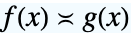 または
または 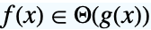 の条件を与える.
AsymptoticEqual[f,g,{x1,…,xn}{ ,…,
,…, }]
}]
{x1,…,xn}{ ,…,
,…, }のときの
}のときの  または
または  の条件を与える.


AsymptoticEqual
AsymptoticEqual[f,g,xx*]
xx*のときの 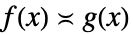 または
または 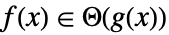 の条件を与える.
AsymptoticEqual[f,g,{x1,…,xn}{ ,…,
,…, }]
}]
{x1,…,xn}{ ,…,
,…, }のときの
}のときの  または
または  の条件を与える.
詳細とオプション
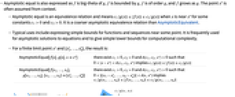
- 「漸近的に等しい」は,f は g の「big-theta」である,f g によって有界である,f は g 程度である,f は g と同じように成長する,等とも表現される.点 x*はコンテキストから推測されることが多い.
- 「漸近的に等しい」は同値関係で,
 かつ
かつ  である定数について,x が x*の近くにあるときに
 ![c_1 TemplateBox[{{g, (, x, )}}, Abs]<=TemplateBox[{{f, (, x, )}}, Abs]<=c_2 TemplateBox[{{g, (, x, )}}, Abs]](Files/AsymptoticEqual.ja/11.png "c_1 TemplateBox[{{g, (, x, )}}, Abs]<=TemplateBox[{{f, (, x, )}}, Abs]<=c_2 TemplateBox[{{g, (, x, )}}, Abs]") であることを意味する.これは,AsymptoticEquivalentよりもきめが粗い漸近的同値関係である.
であることを意味する.これは,AsymptoticEquivalentよりもきめが粗い漸近的同値関係である. - 点の近くの関数や級数の単純な表現のため,方程式の漸近解のため,複雑な計算で単純に下限を表すためにしばしば用いられる.
- 有限極限点の x*および{
 ,…,
,…, }については以下のようになる.
 -
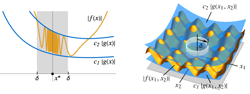
AsymptoticEqual[f[x],g[x],xx*] ![0<TemplateBox[{{x, -, {x, ^, *}}}, Abs]<delta(c_1,c_2,x^*)](Files/AsymptoticEqual.ja/14.png "0<TemplateBox[{{x, -, {x, ^, *}}}, Abs]<delta(c_1,c_2,x^*)") が
が ![c_1 TemplateBox[{{g, (, x, )}}, Abs]<=TemplateBox[{{f, (, x, )}}, Abs]<=c_2 TemplateBox[{{g, (, x, )}}, Abs]](Files/AsymptoticEqual.ja/15.png "c_1 TemplateBox[{{g, (, x, )}}, Abs]<=TemplateBox[{{f, (, x, )}}, Abs]<=c_2 TemplateBox[{{g, (, x, )}}, Abs]") を意味する
を意味する  ,
, ,
,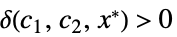 が存在する
が存在するAsymptoticEqual[f[x1,…,xn],g[x1,…,xn],{x1,…,xn}{  ,…,
,…, }]
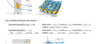
}]![0<TemplateBox[{{{, {{{x, _, 1}, -, {x, _, {(, 1, )}, ^, *}}, ,, ..., ,, {{x, _, n}, -, {x, _, {(, n, )}, ^, *}}}, }}}, Norm]<delta(epsilon,x^*)](Files/AsymptoticEqual.ja/21.png "0<TemplateBox[{{{, {{{x, _, 1}, -, {x, _, {(, 1, )}, ^, *}}, ,, ..., ,, {{x, _, n}, -, {x, _, {(, n, )}, ^, *}}}, }}}, Norm]<delta(epsilon,x^*)") が
が![c_1 TemplateBox[{{g, (, {{x, _, 1}, ,, ..., ,, {x, _, n}}, )}}, Abs]<=TemplateBox[{{f, (, {{x, _, 1}, ,, ..., ,, {x, _, n}}, )}}, Abs]<=c_2 TemplateBox[{{g, (, {{x, _, 1}, ,, ..., ,, {x, _, n}}, )}}, Abs]](Files/AsymptoticEqual.ja/22.png "c_1 TemplateBox[{{g, (, {{x, _, 1}, ,, ..., ,, {x, _, n}}, )}}, Abs]<=TemplateBox[{{f, (, {{x, _, 1}, ,, ..., ,, {x, _, n}}, )}}, Abs]<=c_2 TemplateBox[{{g, (, {{x, _, 1}, ,, ..., ,, {x, _, n}}, )}}, Abs]") を意味する
を意味する  ,
, ,
,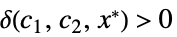 が存在する
が存在する - 無限極限点については以下のようになる.
-
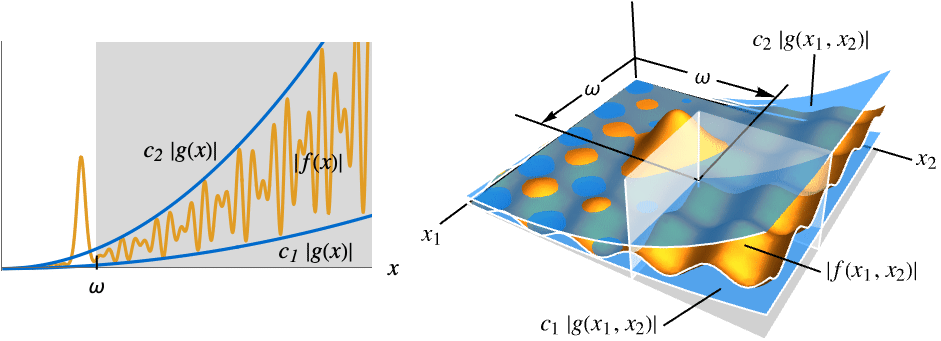
AsymptoticEqual[f[x],g[x],x∞] 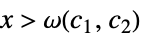 が
が ![c_1 TemplateBox[{{g, (, x, )}}, Abs]<=TemplateBox[{{f, (, x, )}}, Abs]<=c_2 TemplateBox[{{g, (, x, )}}, Abs]](Files/AsymptoticEqual.ja/28.png "c_1 TemplateBox[{{g, (, x, )}}, Abs]<=TemplateBox[{{f, (, x, )}}, Abs]<=c_2 TemplateBox[{{g, (, x, )}}, Abs]") を意味する
を意味する  ,
, ,
,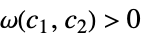 が存在する
が存在するAsymptoticEqual[f[x1,…,xn],g[x1,…,xn],{x1,…,xn}{∞,…,∞}] 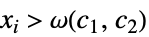 が
が ![c_1 TemplateBox[{{g, (, {{x, _, 1}, ,, ..., ,, {x, _, n}}, )}}, Abs]<=TemplateBox[{{f, (, {{x, _, 1}, ,, ..., ,, {x, _, n}}, )}}, Abs]<=c_2 TemplateBox[{{g, (, {{x, _, 1}, ,, ..., ,, {x, _, n}}, )}}, Abs]](Files/AsymptoticEqual.ja/33.png "c_1 TemplateBox[{{g, (, {{x, _, 1}, ,, ..., ,, {x, _, n}}, )}}, Abs]<=TemplateBox[{{f, (, {{x, _, 1}, ,, ..., ,, {x, _, n}}, )}}, Abs]<=c_2 TemplateBox[{{g, (, {{x, _, 1}, ,, ..., ,, {x, _, n}}, )}}, Abs]") を意味する
を意味する  ,
, ,
,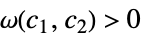 が存在する
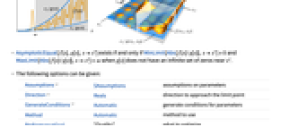
が存在する - g[x]が x*付近に0の無限集合を持たない場合,AsymptoticEqual[f[x],g[x],xx*]は,MinLimit[Abs[f[x]/g[x]],xx*]>0かつMaxLimit[Abs[f[x]/g[x]],xx*]<∞のときかつそのときに限り存在する.
- 次は,使用可能なオプションである.
-
Assumptions $Assumptions パラメータについての仮定 Direction Reals 極限点に近付く方向 GenerateConditions Automatic パラメータについての条件を生成する Method Automatic 使用するメソッド PerformanceGoal "Quality" 何を最適化するか - 次は,Directionの可能な設定である.
-
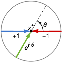
Reals または "TwoSided" 両実数方向から "FromAbove" または -1 上,つまり大きい値から "FromBelow" または +1 下,つまり小さい値から Complexes すべての複素方向から Exp[ θ]  の方向
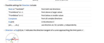
の方向{dir1,…,dirn} 変数 xiに方向 diriを使う - x*におけるDirectionExp[ θ]は,曲線の接線が極限点 x*に近付く方向を示す.
- 次は,GenerateConditionsの可能な設定である.
-
Automatic 一般的ではない条件のみ True すべての条件 False 条件なし None 条件が必要な場合には未評価で返す - PerformanceGoalの可能な設定には,$PerformanceGoal,"Quality","Speed"がある."Quality"設定のとき,Limitはより多くの問題を解いたり,より簡単な結果を与えたりすることが多いが,より多くの時間とメモリが必要になる可能性がある.
例題
すべて開く すべて閉じる



スコープ (9)


![x^2(1-cos(x)) TemplateBox[{{x}}, UnitStepSeq]](Files/AsymptoticEqual.ja/48.png "x^2(1-cos(x)) TemplateBox[{{x}}, UnitStepSeq]")

オプション (9)
Assumptions (1)
Assumptionsを使ってパラメータについての条件を指定する:
Direction (5)
GenerateConditions (3)
デフォルトで,特殊な値でしか結果が無効にならないときは,条件は生成されない:
GenerateConditions->Trueのときは,それら一般的ではない条件さえもがレポートされる:
アプリケーション (10)
基本的なアプリケーション (5)









計算の複雑性 (3)
バブルソートでは,隣接近傍が比較され,順序が狂っている場合には入れ替えられる.1回のパス(n-1 回の比較)の後で最大要素が末尾になる.このプロセスが残りの n-1個の要素に対して行われ,先頭の2つの要素が残るまでこれが繰り返される.比較と入替えが c ステップだとすると,ソートのステップ総数は次のようになる:
 であり,したがってこのアルゴリズムのランタイムが2次であることを示す:
マージソートでは,要素のリストが2つに分割され,半分ずつソートされ,最後に2つの部分が結合される.であるから,ソート時間T[n]は中間を計算する一定の時間 b,各半分を計算する時間2T[n/2],2つの半分を結合するための要素数の倍数 a n の合計になる:
再帰方程式を解いて n 個の要素をソートする時間 t を求める:
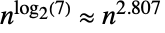
 であり,したがってこのアルゴリズムのランタイムが
  であることを示す:
シュトラッセン(Strassen)のアルゴリズムは,はじめて求まったSubcubic行列の乗法アルゴリズムである.このアルゴリズムは,2つの  行列のそれぞれをサイズが等しい4つの部分行列に分割し,8つの部分行列から14個の特定の線形結合を形成し,これらの7対の乗算を行なって,7つの結果の線形結合を形成する,という4ステップからなる.乗算を行う時間
  は,したがって,行列を分割する固定時間
  ,2番目と4番目の線形結合を形成する時間
  ,第3ステップの
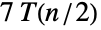 である:
である:
収束判定法 (2)
![sum_(n=1)^inftyTemplateBox[{{a, _, n}}, Abs]<infty](Files/AsymptoticEqual.ja/72.png "sum_(n=1)^inftyTemplateBox[{{a, _, n}}, Abs]<infty") であれば,列
であれば,列  は絶対加算可能であると言われる.第2列が
  なら,比較判定法は,
 が絶対加算可能であるときかつそのときに限りみ
  も絶対加算可能であると述べる.この判定法を使って,
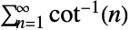
 総和と比較することによって
  が収束することを示す:
SumConvergenceが与える答と比較する:



SumConvergenceが与える答と比較する:
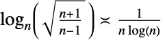
![int_a^bTemplateBox[{{f, , {(, x, )}}}, Abs]dx<infty](Files/AsymptoticEqual.ja/84.png "int_a^bTemplateBox[{{f, , {(, x, )}}}, Abs]dx<infty") ならば,関数
ならば,関数  は
は に対して完全に積分可能であると言われる.
 と
と  が開区間
が開区間 で連続的であり,
 と
と  の両方で
の両方で  なら,比較判定法は
  が完全に積分可能であるときかつそのときに限り
  もそうであるとする.この判定法を使って
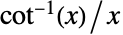 が
が で完全に積分可能であることを示す:


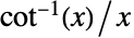
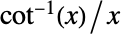 が
が 上では積分可能ではないことは,これを
 と比較することで示すことができる:






![TemplateBox[{x}, LogIntegral]/x](Files/AsymptoticEqual.ja/109.png "TemplateBox[{x}, LogIntegral]/x")
特性と関係 (6)
AsymptoticEqualは同値関係,つまり反射的(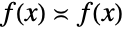 )である:
)である:
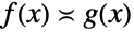
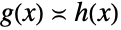
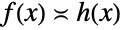
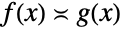
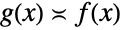
MaxLimit[Abs[f[x]/g[x]],xx0]<∞かつMinLimit[Abs[f[x]/g[x]],xx0]>0のときかつそのときに限りAsymptoticEqual[f[x],g[x],xx0]である:
0<Limit[Abs[f[x]/g[x]],xx0]<∞であればAsymptoticEqual[f[x],g[x],xx0]である:
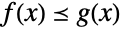
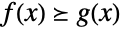
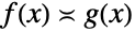
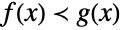
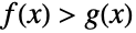
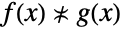
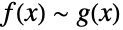
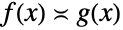
逆は偽である.したがって,AsymptoticEqualはAsymptoticEquivalentより粗いと言える:
テキスト
Wolfram Research (2018), AsymptoticEqual, Wolfram言語関数, https://reference.wolfram.com/language/ref/AsymptoticEqual.html.
CMS
Wolfram Language. 2018. "AsymptoticEqual." Wolfram Language & System Documentation Center. Wolfram Research. https://reference.wolfram.com/language/ref/AsymptoticEqual.html.
APA
Wolfram Language. (2018). AsymptoticEqual. Wolfram Language & System Documentation Center. Retrieved from https://reference.wolfram.com/language/ref/AsymptoticEqual.html