AsymptoticEqual[f,g,xx*]
给出当 xx* 时 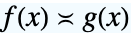 或
或 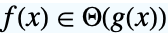 的条件.
的条件.
AsymptoticEqual[f,g,{x1,…,xn}{ ,…,
,…, }]
}]
给出当 {x1,…,xn}{ ,…,
,…, } 时
} 时  或
或  的条件.
的条件.


AsymptoticEqual
AsymptoticEqual[f,g,xx*]
给出当 xx* 时 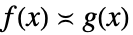 或
或 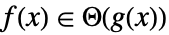 的条件.
的条件.
AsymptoticEqual[f,g,{x1,…,xn}{ ,…,
,…, }]
}]
给出当 {x1,…,xn}{ ,…,
,…, } 时
} 时  或
或  的条件.
的条件.
更多信息和选项
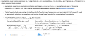
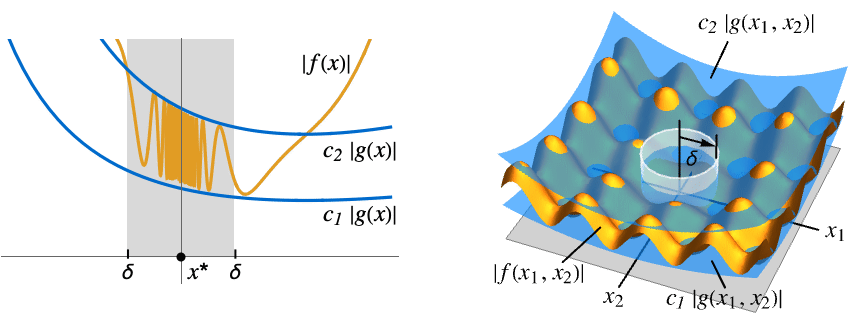
- 渐近相等也被表示为 f 是 g 的大写的 theta,f 由 g 限定,f 的大小大约为 g,f 随 g 增长. 经常从上下文中估计点 x*.
- 渐近相等是一种等价关系,意味着对于某些常数
 和
和  ,当 x 靠近 x* 时,
 ![c_1 TemplateBox[{{g, (, x, )}}, Abs]<=TemplateBox[{{f, (, x, )}}, Abs]<=c_2 TemplateBox[{{g, (, x, )}}, Abs]](Files/AsymptoticEqual.zh/11.png "c_1 TemplateBox[{{g, (, x, )}}, Abs]<=TemplateBox[{{f, (, x, )}}, Abs]<=c_2 TemplateBox[{{g, (, x, )}}, Abs]") . 它是比 AsymptoticEquivalent 更粗略的一种渐近等价关系.
. 它是比 AsymptoticEquivalent 更粗略的一种渐近等价关系. - 典型的用途包括表示函数和序列在一些点附近的简单界限. 它经常用于方程的渐近解,并给出计算复杂度的简单下界.
- 对于有限极限点 x* 和 {
 ,…,
,…, },结果为:
 -
AsymptoticEqual[f[x],g[x],xx*] 存在  、
、 和
和 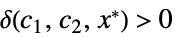 ,使得
,使得 ![0<TemplateBox[{{x, -, {x, ^, *}}}, Abs]<delta(c_1,c_2,x^*)](Files/AsymptoticEqual.zh/17.png "0<TemplateBox[{{x, -, {x, ^, *}}}, Abs]<delta(c_1,c_2,x^*)") 意味着
意味着 ![c_1 TemplateBox[{{g, (, x, )}}, Abs]<=TemplateBox[{{f, (, x, )}}, Abs]<=c_2 TemplateBox[{{g, (, x, )}}, Abs]](Files/AsymptoticEqual.zh/18.png "c_1 TemplateBox[{{g, (, x, )}}, Abs]<=TemplateBox[{{f, (, x, )}}, Abs]<=c_2 TemplateBox[{{g, (, x, )}}, Abs]") 成立
成立AsymptoticEqual[f[x1,…,xn],g[x1,…,xn],{x1,…,xn}{  ,…,
,…, }]
}]存在  、
、 和
和 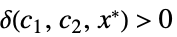 ,使得
,使得 ![0<TemplateBox[{{{, {{{x, _, 1}, -, {x, _, {(, 1, )}, ^, *}}, ,, ..., ,, {{x, _, n}, -, {x, _, {(, n, )}, ^, *}}}, }}}, Norm]<delta(epsilon,x^*)](Files/AsymptoticEqual.zh/24.png "0<TemplateBox[{{{, {{{x, _, 1}, -, {x, _, {(, 1, )}, ^, *}}, ,, ..., ,, {{x, _, n}, -, {x, _, {(, n, )}, ^, *}}}, }}}, Norm]<delta(epsilon,x^*)") 意味着
意味着 ![c_1 TemplateBox[{{g, (, {{x, _, 1}, ,, ..., ,, {x, _, n}}, )}}, Abs]<=TemplateBox[{{f, (, {{x, _, 1}, ,, ..., ,, {x, _, n}}, )}}, Abs]<=c_2 TemplateBox[{{g, (, {{x, _, 1}, ,, ..., ,, {x, _, n}}, )}}, Abs]](Files/AsymptoticEqual.zh/25.png "c_1 TemplateBox[{{g, (, {{x, _, 1}, ,, ..., ,, {x, _, n}}, )}}, Abs]<=TemplateBox[{{f, (, {{x, _, 1}, ,, ..., ,, {x, _, n}}, )}}, Abs]<=c_2 TemplateBox[{{g, (, {{x, _, 1}, ,, ..., ,, {x, _, n}}, )}}, Abs]") 成立
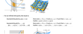
成立 - 对于无限极限点,结果为:
-
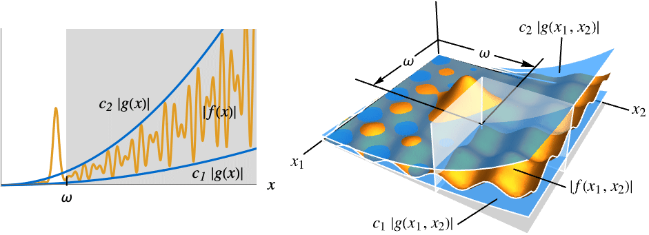
AsymptoticEqual[f[x],g[x],x∞] 存在  、
、 和
和 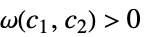 ,使得
,使得 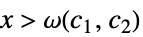 意味着
意味着 ![c_1 TemplateBox[{{g, (, x, )}}, Abs]<=TemplateBox[{{f, (, x, )}}, Abs]<=c_2 TemplateBox[{{g, (, x, )}}, Abs]](Files/AsymptoticEqual.zh/31.png "c_1 TemplateBox[{{g, (, x, )}}, Abs]<=TemplateBox[{{f, (, x, )}}, Abs]<=c_2 TemplateBox[{{g, (, x, )}}, Abs]") 成立
成立AsymptoticEqual[f[x1,…,xn],g[x1,…,xn],{x1,…,xn}{∞,…,∞}] 存在  、
、 和
和 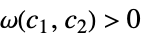 ,使得
,使得 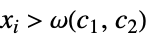 意味着
意味着 ![c_1 TemplateBox[{{g, (, {{x, _, 1}, ,, ..., ,, {x, _, n}}, )}}, Abs]<=TemplateBox[{{f, (, {{x, _, 1}, ,, ..., ,, {x, _, n}}, )}}, Abs]<=c_2 TemplateBox[{{g, (, {{x, _, 1}, ,, ..., ,, {x, _, n}}, )}}, Abs]](Files/AsymptoticEqual.zh/36.png "c_1 TemplateBox[{{g, (, {{x, _, 1}, ,, ..., ,, {x, _, n}}, )}}, Abs]<=TemplateBox[{{f, (, {{x, _, 1}, ,, ..., ,, {x, _, n}}, )}}, Abs]<=c_2 TemplateBox[{{g, (, {{x, _, 1}, ,, ..., ,, {x, _, n}}, )}}, Abs]") 成立
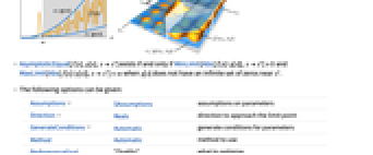
成立 - 在 x* 附近 g[x] 的值不为无限个零时,当且仅当 MinLimit[Abs[f[x]/g[x]],xx*]>0 和 MaxLimit[Abs[f[x]/g[x]],xx*]<∞ 成立时,AsymptoticEqual[f[x],g[x],xx*] 才存在.
- 可以给出下列选项:
-
Assumptions $Assumptions 对参数的设定 Direction Reals 趋近极限点的方向 GenerateConditions Automatic 对参数生成条件 Method Automatic 所使用的方法 PerformanceGoal "Quality" 优化目标 - Direction 的可能设置包括:
-
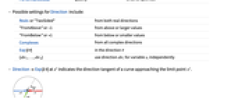
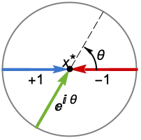
Reals or "TwoSided" 从两个实方向 "FromAbove" or -1 从上面或较大的值 "FromBelow" or +1 从下面或较小的值 Complexes 从所有复方向 Exp[ θ] 从方向 
{dir1,…,dirn} 对变量 xi 分别使用方向 diri - 在 x* 处的 DirectionExp[ θ] 表示接近极限点 x* 的曲线的方向切线.
- GenerateConditions 的可能设置包括:
-
Automatic 只给出非通用条件 True 所有条件 False 不给出条件 None 如果需要条件则不经计算直接返回 - PerformanceGoal 的可能设置包括 $PerformanceGoal、"Quality" 和 "Speed". 当设置为 "Quality" 时,AsymptoticEqual 通常可以解出更多的问题或者产生更简单的结果,但是可能会耗费更多的时间和内存.
范例
打开所有单元 关闭所有单元



范围 (9)


![x^2(1-cos(x)) TemplateBox[{{x}}, UnitStepSeq]](Files/AsymptoticEqual.zh/48.png "x^2(1-cos(x)) TemplateBox[{{x}}, UnitStepSeq]")

选项 (9)
Assumptions (1)
用 Assumptions 为参数指定条件:
Direction (5)
GenerateConditions (3)
当 GenerateConditions->True 时,非通用条件也要报告:
应用 (10)
基本应用 (5)









计算复杂度 (3)
在冒泡排序中,对相邻的项进行比较,如果顺序不对即进行交换. 经过 n-1 次比较后,最大的元素在最后. 然后在剩余的 n-1 个元素上重复该过程,直到开头处只剩下两个元素. 如果比较和交换需要 c 个步骤,则排序需要的总步骤如下所示:

在合并排序中,元素列表被分成两部分,分别对每部分进行排序,然后合并两个部分. 因此,进行排序的总时间 T[n] 将是用于计算中值的某个固定时间 b 加上对每一半元素进行排序的时间 2T[n/2],再加上用于将两部分元素合并在一起的时间,即元素个数的倍数 a n:


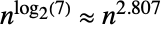
Strassen 算法是第一个发现的 subcubic 矩阵乘法算法. 它由 4 个步骤组成:将两个  矩阵中的每一个分成 4 个大小相等的子矩阵,从 8 个子矩阵中形成 14 个特定的线性组合,将 7 对这样的组合相乘,形成 7 个结果的线性组合. 因此,执行乘法的时间
  将是用于分割矩阵的固定定时间
  ,在第二和第四步中形成线性组合的时间则为
  ,第三步花费的时间则为
 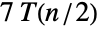 :
:
收敛性测试 (2)
如果 ![sum_(n=1)^inftyTemplateBox[{{a, _, n}}, Abs]<infty](Files/AsymptoticEqual.zh/72.png "sum_(n=1)^inftyTemplateBox[{{a, _, n}}, Abs]<infty") ,序列
,序列  被认为是绝对可以求和的. 如果第二个序列
  ,比较测试指出,当且仅当
  是绝对可以求和的,
 才是绝对可以求和的. 通过与
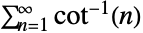
  的和进行比较,用测试证明
  收敛:
收敛:
与 SumConvergence 给出的答案比较:



与 SumConvergence 给出的答案比较:
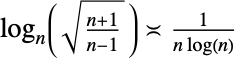
如果 ![int_a^bTemplateBox[{{f, , {(, x, )}}}, Abs]dx<infty](Files/AsymptoticEqual.zh/84.png "int_a^bTemplateBox[{{f, , {(, x, )}}}, Abs]dx<infty") ,函数
,函数  被认为在
被认为在  上是绝对可积的. 如果
  和
和  在开区间
在开区间  上是连续的,且在
  和
和  处有
处有  ,比较测试指出,当且仅当
  是绝对可积的,
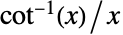
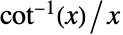
 才是绝对可积的. 用测试证明
 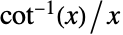 在
在  上是绝对可积的:










![TemplateBox[{x}, LogIntegral]/x](Files/AsymptoticEqual.zh/109.png "TemplateBox[{x}, LogIntegral]/x")
属性和关系 (6)
AsymptoticEqual 是一种等价关系,意味着它是自反的(即 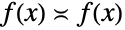 ):
):
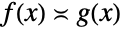
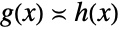
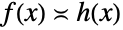
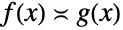
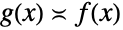
当且仅当 MaxLimit[Abs[f[x]/g[x]],xx0]<∞ 和 MinLimit[Abs[f[x]/g[x]],xx0]>0 时,AsymptoticEqual[f[x],g[x],xx0] 的结果为:
如果 0<Limit[Abs[f[x]/g[x]],xx0]<∞,则 AsymptoticEqual[f[x],g[x],xx0] 的结果为:
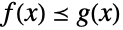
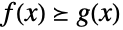
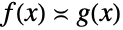
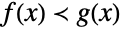
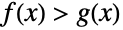
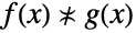
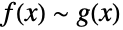
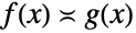
但反过来不成立,所以 AsymptoticEqual 没有 AsymptoticEquivalent 严格:
文本
Wolfram Research (2018),AsymptoticEqual,Wolfram 语言函数,https://reference.wolfram.com/language/ref/AsymptoticEqual.html.
CMS
Wolfram 语言. 2018. "AsymptoticEqual." Wolfram 语言与系统参考资料中心. Wolfram Research. https://reference.wolfram.com/language/ref/AsymptoticEqual.html.
APA
Wolfram 语言. (2018). AsymptoticEqual. Wolfram 语言与系统参考资料中心. 追溯自 https://reference.wolfram.com/language/ref/AsymptoticEqual.html 年