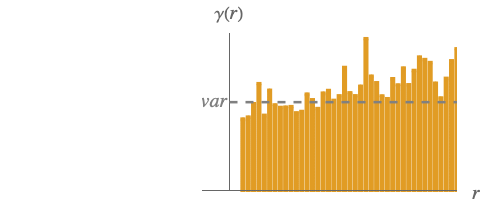
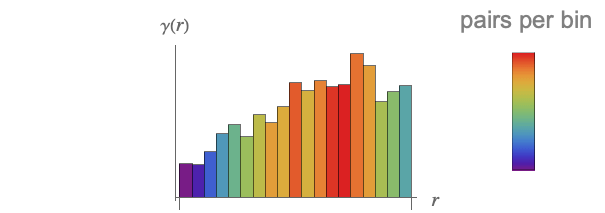
BinnedVariogramList[{loc1val1,loc2val2,…}]
ビニングされた値を使ってバリオグラムを計算する.
BinnedVariogramList[{loc1,loc2,…}{val1,val2,…}]
同じ結果を生成する.
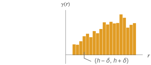
BinnedVariogramList[…,spec]
HistogramListで与えられているようにビニング spec を指定することを許容する.
BinnedVariogramList
BinnedVariogramList[{loc1val1,loc2val2,…}]
ビニングされた値を使ってバリオグラムを計算する.
BinnedVariogramList[{loc1,loc2,…}{val1,val2,…}]
同じ結果を生成する.
BinnedVariogramList[…,spec]
HistogramListで与えられているようにビニング spec を指定することを許容する.
詳細とオプション
- BinnedVariogramListは,経験バリオグラムあるいは標本バリオグラムとしても知られている.
- BinnedVariogramListは,通常は,データにおける空間データ依存の初期評価を得るために使われる.また,高品質のEstimatedVariogramModelの第1ステージとしても使われる.
- 場所
と
における空間過程
のバリオグラム
は
で与えられる.これは,過程が空間的にどの程度の速さで変化するかを測定する. - 過程が弱定常のとき,バリオグラムは場所の差,つまり

だけに依存する.過程が等方性のときは,バリオグラムは
である場所の間の距離
だけに依存する.
の値
は
として計算できる.ただし,
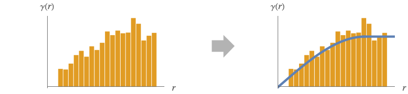
である.結果はビニングされたバリオグラムである.- 結果のビニングされたバリオグラムは,通常は,有効なバリオグラムではない.

で場所 piとなるように,すべての重み wiに対して条件付きで負の定性
である必要がある.しかし,EstimatedVariogramModelで行われるように,これを使って有効なバリオグラムであるバリオグラムモデルをフィットすることができる. - ビニングされたバリオグラムからデータにトレンドがあるかどうかが検出できるが,これは非有界のバリオグラムになる.
- 次は,使用可能なオプションである.
-
DistanceFunction Automatic 距離を計算する関数を指定する Method "NonLattice" ビニングする場所の形状を指定する SpatialTrendFunction None グローバルトレンドモデルを指定する - Methodには次の設定が使える.
-
"NonLattice" 場所は集合として与えられる - 次は,使用可能なMethodオプションである.
-
"BinCenter" "Centroid" ビンの中心の計算方法 "MaxDistanceRatio" 1/3 最大ペアの距離に対する距離の比率がそれより大きいと削除されるデータペア "MinPairs" 30 含んでいるペアがそれより少ないと削除されるビン "ScaleEstimator" "Cressie" 使用するスケール推定器 - "ScaleEstimator"には以下の設定を使うことができる.
-
"Cressie" 平方根の四次モーメントを使う "Matheron" 二次モーメントを使う "Qn" QnDispersionを使う "Sn" SnDispersionを使う - BinnedVariogramは,重みが各距離ビンについてのペアの数である二次元WeightedDataを返す.
例題
すべて開く すべて閉じる例 (2)
データからBinnedVariogramListを計算する:
locations = {...};
vals = {...};PointValuePlot[locations -> vals]BinnedVariogramList[locations -> vals]ListPlot[%, Filling -> Axis]データからBinnedVariogramListを計算する:
data = ResourceData["Sample Data: US Ozone 2021"]PointValuePlot[data, ColorFunction -> "Rainbow"]BinnedVariogramList[data -> "Ozone"]ListPlot[%, Filling -> Axis]スコープ (3)
基本的な用法 (3)
場所と値のペアのリストについてビニングされたバリオグラムを計算する:
data = {...};data[[ ;; 2]]PointValuePlot[data, PlotLegends -> Automatic]bv = BinnedVariogramList[data]重みで各距離のビンのペアの数を表してビニングされたバリオグラムを可視化する:
PointValuePlot[bv["InputData"] -> bv["InputWeights"], ColorFunction -> "Rainbow", PlotLegends -> Automatic]ビニングにHistogramListスペックを使う:
SeedRandom["bingo"];
locations = RandomPoint[Disk[], 100];
values = Exp[-Total /@ locations] + RandomReal[1, 100];PointValuePlot[locations -> values, PlotLegends -> Automatic]ビニングされたバリオグラムをAutomaticビン指定で計算する:
ev0 = BinnedVariogramList[locations -> values];ev1 = BinnedVariogramList[locations -> values, 5];ev2 = BinnedVariogramList[locations -> values, {.01}];名前付きのビニング法を使う(デフォルトはScott法である):
ev3 = BinnedVariogramList[locations -> values, "Knuth"];ListLinePlot[{ev0, ev1, ev2, ev3}, PlotRange -> All, PlotLegends -> {"ev0", "ev1", "ev2", "ev3"}]地理データのBinnedVariogramListを計算する:
locs = GeoPosition[{{25.5, -124.5}, {25.5, -123.5}, {25.5, -122.5}, {25.5, -121.5}, {25.5, -120.5},
{25.5, -112.5}, {25.5, -111.5}, {25.5, -110.5}, {25.5, -109.5}, {25.5, -108.5}, {25.5, -107.5},
{25.5, -106.5}, {25.5, -105.5}, {25.5, -104.5}, {25.5 ... 8.5, -87.5}, {48.5, -86.5},
{48.5, -85.5}, {48.5, -84.5}, {48.5, -83.5}, {48.5, -82.5}, {48.5, -81.5}, {48.5, -80.5},
{48.5, -79.5}, {48.5, -78.5}, {48.5, -72.5}, {48.5, -71.5}, {48.5, -70.5}, {48.5, -69.5},
{48.5, -68.5}, {48.5, -67.5}}];ozone = {...};PointValuePlot[locs -> ozone, ColorFunction -> "Rainbow"]bv = BinnedVariogramList[locs -> ozone]ListPlot[bv, AxesLabel -> {"m"}]オプション (7)
DistanceFunction (1)
非地理的な場所については,異なるDistanceFunctionを使うことができる:
locs = {...};
vals = {...};bv1 = BinnedVariogramList[locs -> vals, DistanceFunction -> ManhattanDistance]EuclideanDistanceはデカルト座標のデフォルトの距離関数である:
bv2 = BinnedVariogramList[locs -> vals, DistanceFunction -> EuclideanDistance]bv3 = BinnedVariogramList[locs -> vals, DistanceFunction -> (Norm[#1 - #2, 3]&)]ListPlot[{bv1, bv2, bv3}, PlotStyle -> PointSize[0.015], PlotLegends -> {"p = 1", "p = 2", "p = 3"}]Method (5)
Method (1)
BinCenter (1)
さまざまな"BinCenter"指定についてBinnedVariogramListを計算する:
data = RandomPointConfiguration[MaternPointProcess[50, 20, .1, 2], Rectangle[]]["Points"];
vals = Sin[Norm /@ data];PointValuePlot[data -> vals, PlotLegends -> Automatic]center = {"Centroid", Mean, SpatialMedian};res = Map[BinnedVariogramList[data -> vals, Method -> {"NonLattice", "BinCenter" -> #}]&, center]ListPlot[res, PlotStyle -> PointSize[.02], PlotRange -> All, PlotLegends -> center]MaxDistanceRatio (1)
さまざまな"MaxDistanceRatio"設定についてBinnedVariogramListを計算する:
data = RandomReal[1, {200, 2}];
vals = Sin[Norm /@ data];PointValuePlot[data -> vals, PlotLegends -> Automatic]mdr = {.2, .4, .6, .8};res = Map[BinnedVariogramList[data -> vals, Method -> {"NonLattice", "MaxDistanceRatio" -> #}]&, mdr]ListPlot[First[#], PlotRange -> {{0, .9}, {0, .1}}, PlotStyle -> PointSize[0.02], PlotLabel -> Last[#], ImageSize -> 200]& /@ Transpose[{res, mdr}]MinPairs (1)
さまざまな"MinPairs"指定についてBinnedVariogramListを計算する:
data = RandomReal[1, {100, 2}];
vals = Sin[Norm /@ data];PointValuePlot[data -> vals, PlotLegends -> Automatic]mp = {10, 50, 80, 100};res = Map[BinnedVariogramList[data -> vals, Method -> {"NonLattice", "MinPairs" -> #}]&, mp]ListPlot[First[#], PlotRange -> {{0, .5}, All}, PlotLabel -> Last[#], Ticks -> {{0, .1, .2, .3}, {0, .01, .02, .03}}, ImageSize -> 200]& /@ Transpose[{res, mp}]ScaleEstimator (1)
さまざまな"ScaleEstimator"指定についてBinnedVariogramListを計算する:
data = RandomReal[1, {500, 2}];
vals = Sin[Norm /@ data];PointValuePlot[data -> vals, PlotLegends -> Automatic]est = {"Cressie", "Matheron", "Qn", "Sn"};res = Map[BinnedVariogramList[data -> vals, Method -> {Automatic, "ScaleEstimator" -> #}]&, est]ListPlot[res, PlotLegends -> est]SpatialTrendFunction (1)
デフォルトで,BinnedVariogramListはトレンドを仮定しないが,データからは自動的にトレンドが除去できる:
SeedRandom["bingo"];
locs = RandomPoint[Disk[], 100];
vals = Exp[-Total /@ locs] + RandomReal[1, 100];PointValuePlot[locs -> vals, PlotLegends -> Automatic]SpatialTrendFunctionを使ってトレンド設定を指定し,ビニングされたバリオグラムを計算する:
trends = {1, 2, (1 / Exp[Total@#]&)};
res = Map[BinnedVariogramList[locs -> vals, SpatialTrendFunction -> #]&, trends]このプロットは,データに少なくとも一次のトレンドがあることを示している:
ListLinePlot[res, PlotLegends -> trend]アプリケーション (2)
ビニングされたバリオグラムを使ってEstimatedVariogramModelの初期の視覚形状のアイディアを得ることができる:
data = ResourceData["Sample Data: US Ozone 2021"]注釈キーで指定された値についてビニングされたバリオグラムを計算する:
bv = BinnedVariogramList[data -> "Ozone"]ListPlot[bv]models = {"Cubic", "Spherical", "Gaussian", "Askey"};vars = Map[EstimatedVariogramModel[data -> "Ozone", #]&, models];Grid[Partition[MapThread[#1["Visualization", PlotLabel -> #2]&, {vars, models}], 2]]BinnedVariogramListを使ってデータにトレンドがあることを示すことができる:
SeedRandom["trendy"];
locs = RandomPoint[Disk[], 100];
vals = Exp[-Total /@ locs] + RandomReal[1, 100];PointValuePlot[locs -> vals, PlotLegends -> Automatic]bv0 = BinnedVariogramList[locs -> vals]ListLinePlot[bv0]bv1 = BinnedVariogramList[locs -> vals, SpatialTrendFunction -> 1]線形にトレンドを除去したビニングされたバリオグラムをデフォルトと比較する:
ListLinePlot[{bv0, bv1}, PlotLegends -> {"no trend", "linear trend"}]考えられる問題 (1)
BinnedVariogramListは,ビンごとのペアの最小数を満たすのに十分なデータがなければ失敗する:

locs = RandomReal[1, {4, 2}];
vals = RandomReal[1, 4];BinnedVariogramList[locs -> vals]関連するガイド
-
▪
- 空間推定
テキスト
Wolfram Research (2021), BinnedVariogramList, Wolfram言語関数, https://reference.wolfram.com/language/ref/BinnedVariogramList.html.
CMS
Wolfram Language. 2021. "BinnedVariogramList." Wolfram Language & System Documentation Center. Wolfram Research. https://reference.wolfram.com/language/ref/BinnedVariogramList.html.
APA
Wolfram Language. (2021). BinnedVariogramList. Wolfram Language & System Documentation Center. Retrieved from https://reference.wolfram.com/language/ref/BinnedVariogramList.html
BibTeX
@misc{reference.wolfram_2026_binnedvariogramlist, author="Wolfram Research", title="{BinnedVariogramList}", year="2021", howpublished="\url{https://reference.wolfram.com/language/ref/BinnedVariogramList.html}", note=[Accessed: 08-September-2026]}
BibLaTeX
@online{reference.wolfram_2026_binnedvariogramlist, organization={Wolfram Research}, title={BinnedVariogramList}, year={2021}, url={https://reference.wolfram.com/language/ref/BinnedVariogramList.html}, note=[Accessed: 08-September-2026]}