

BinnedVariogramList
BinnedVariogramList[{loc1val1,loc2val2,…}]
使用分箱值计算变异函数.
BinnedVariogramList[{loc1,loc2,…}{val1,val2,…}]
生成相同的结果.
BinnedVariogramList[…,spec]
允许指定 HistogramList 中给出的分箱规范 spec.
更多信息和选项
- BinnedVariogramList 也称为经验变异函数或样本变异函数.
- BinnedVariogramList 通常用于对数据中的空间数据依赖性进行初步评估. 它还用于估计高质量 EstimatedVariogramModel 的第一阶段.
- 在位置
 和
和  的空间过程
的空间过程  的变异函数
的变异函数  由
由  给出. 它衡量过程在空间上变化的速度.
 - 当过程弱平稳时,变异函数仅取决于位置的差异,即
 . 当过程各向同性时,它只取决于位置
  之间的距离,其中
 ![h=TemplateBox[{{{p, _, 1}, -, {p, _, 2}}}, Norm]](Files/BinnedVariogramList.zh/8.png "h=TemplateBox[{{{p, _, 1}, -, {p, _, 2}}}, Norm]") .
. - 对于
 ,
, 的值由
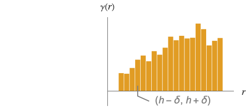
的值由 ![1/(2 TemplateBox[{S}, Abs])sum_({p,q} in S)(x(p)-x(q))^2](Files/BinnedVariogramList.zh/11.png "1/(2 TemplateBox[{S}, Abs])sum_({p,q} in S)(x(p)-x(q))^2") 计算,其中
计算,其中 ![S={{p,q}|h-delta<=TemplateBox[{{p, -, q}}, Norm]<h+delta}](Files/BinnedVariogramList.zh/12.png "S={{p,q}|h-delta<=TemplateBox[{{p, -, q}}, Norm]<h+delta}") . 结果是一个分箱变异函数:
. 结果是一个分箱变异函数: - 生成的分箱变异函数通常不是有效的变异函数. 对于满足
 的所有权值 wi 和位置pi,它需要有条件的负定
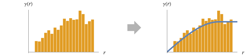
 ![sum_(i=1)^nsum_(j=1)^nw_i w_j gamma(TemplateBox[{{{p, _, i}, -, {p, _, j}}}, Norm])<=0](Files/BinnedVariogramList.zh/15.png "sum_(i=1)^nsum_(j=1)^nw_i w_j gamma(TemplateBox[{{{p, _, i}, -, {p, _, j}}}, Norm])<=0") . 然而,它可用于拟合将成为有效变异函数的变异函数模型,正如在 EstimatedVariogramModel 中所做的那样.
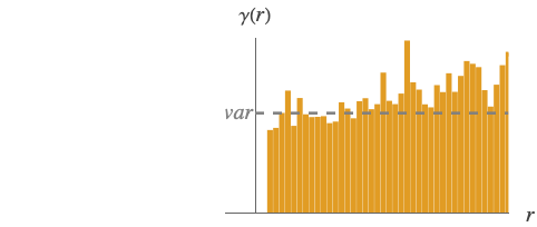
. 然而,它可用于拟合将成为有效变异函数的变异函数模型,正如在 EstimatedVariogramModel 中所做的那样. - 从分箱变异函数中,可以检测数据中是否存在导致无界变异函数的趋势.
- 可以提供以下选项:
-
DistanceFunction Automatic 指定计算距离的函数 Method "NonLattice" 指定用于分箱的位置形状 SpatialTrendFunction None 指定全局趋势模型 - 以下设置可用于 Method:
-
"NonLattice" 位置以集合的形式给出 - 可使用下列 Method 选项:
-
"BinCenter" "Centroid" 如何计算箱的中心 "MaxDistanceRatio" 1/3 距离与最大距离对之比较大的数据对被丢弃 "MinPairs" 30 包含较少对的箱被丢弃 "ScaleEstimator" "Cressie" 使用哪个缩放估计器 - 以下设置可用于 "ScaleEstimator":
-
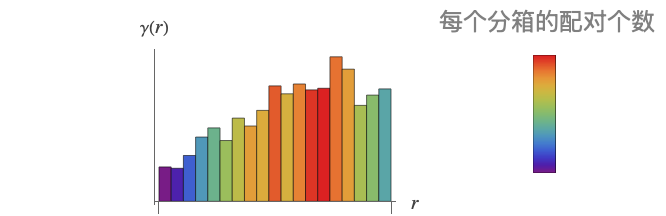
"Cressie" 使用平方根的四阶矩 "Matheron" 使用二阶矩 "Qn" 使用 QnDispersion "Sn" 使用 SnDispersion - BinnedVariogram 返回二维 WeightedData,权值是每个距离箱对的个数.
范例
打开所有单元 关闭所有单元基本范例 (2)
由数据计算 BinnedVariogramList:
locations = {...};
vals = {...};PointValuePlot[locations -> vals]BinnedVariogramList[locations -> vals]ListPlot[%, Filling -> Axis]从地理数据计算 BinnedVariogramList:
data = ResourceData["Sample Data: US Ozone 2021"]PointValuePlot[data, ColorFunction -> "Rainbow"]BinnedVariogramList[data -> "Ozone"]ListPlot[%, Filling -> Axis]范围 (3)
基本用法 (3)
data = {...};data[[ ;; 2]]PointValuePlot[data, PlotLegends -> Automatic]bv = BinnedVariogramList[data]PointValuePlot[bv["InputData"] -> bv["InputWeights"], ColorFunction -> "Rainbow", PlotLegends -> Automatic]使用 HistogramList 规范进行分箱:
SeedRandom["bingo"];
locations = RandomPoint[Disk[], 100];
values = Exp[-Total /@ locations] + RandomReal[1, 100];PointValuePlot[locations -> values, PlotLegends -> Automatic]使用 Automatic 分箱规范计算分箱变异函数:
ev0 = BinnedVariogramList[locations -> values];ev1 = BinnedVariogramList[locations -> values, 5];ev2 = BinnedVariogramList[locations -> values, {.01}];ev3 = BinnedVariogramList[locations -> values, "Knuth"];ListLinePlot[{ev0, ev1, ev2, ev3}, PlotRange -> All, PlotLegends -> {"ev0", "ev1", "ev2", "ev3"}]计算地理数据的 BinnedVariogramList:
locs = GeoPosition[{{25.5, -124.5}, {25.5, -123.5}, {25.5, -122.5}, {25.5, -121.5}, {25.5, -120.5},
  {25.5, -112.5}, {25.5, -111.5}, {25.5, -110.5}, {25.5, -109.5}, {25.5, -108.5}, {25.5, -107.5},
  {25.5, -106.5}, {25.5, -105.5}, {25.5, -104.5}, {25.5 ... 8.5, -87.5}, {48.5, -86.5},
  {48.5, -85.5}, {48.5, -84.5}, {48.5, -83.5}, {48.5, -82.5}, {48.5, -81.5}, {48.5, -80.5},
  {48.5, -79.5}, {48.5, -78.5}, {48.5, -72.5}, {48.5, -71.5}, {48.5, -70.5}, {48.5, -69.5},
{48.5, -68.5}, {48.5, -67.5}}];ozone = {...};PointValuePlot[locs -> ozone, ColorFunction -> "Rainbow"]bv = BinnedVariogramList[locs -> ozone]ListPlot[bv, AxesLabel -> {"m"}]选项 (7)
DistanceFunction (1)
对于非地理位置,可以使用不同的 DistanceFunction:
locs = {...};
vals = {...};bv1 = BinnedVariogramList[locs -> vals, DistanceFunction -> ManhattanDistance]EuclideanDistance 是笛卡尔坐标的默认距离函数:
bv2 = BinnedVariogramList[locs -> vals, DistanceFunction -> EuclideanDistance]bv3 = BinnedVariogramList[locs -> vals, DistanceFunction -> (Norm[#1 - #2, 3]&)]ListPlot[{bv1, bv2, bv3}, PlotStyle -> PointSize[0.015], PlotLegends -> {"p = 1", "p = 2", "p = 3"}]Method (5)
Method (1)
BinCenter (1)
计算不同 "BinCenter" 规范的 BinnedVariogramList:
data = RandomPointConfiguration[MaternPointProcess[50, 20, .1, 2], Rectangle[]]["Points"];
vals = Sin[Norm /@ data];PointValuePlot[data -> vals, PlotLegends -> Automatic]center = {"Centroid", Mean, SpatialMedian};res = Map[BinnedVariogramList[data -> vals, Method -> {"NonLattice", "BinCenter" -> #}]&, center]ListPlot[res, PlotStyle -> PointSize[.02], PlotRange -> All, PlotLegends -> center]MaxDistanceRatio (1)
计算不同 "MaxDistanceRatio" 规范的 BinnedVariogramList:
data = RandomReal[1, {200, 2}];
vals = Sin[Norm /@ data];PointValuePlot[data -> vals, PlotLegends -> Automatic]mdr = {.2, .4, .6, .8};res = Map[BinnedVariogramList[data -> vals, Method -> {"NonLattice", "MaxDistanceRatio" -> #}]&, mdr]ListPlot[First[#], PlotRange -> {{0, .9}, {0, .1}}, PlotStyle -> PointSize[0.02], PlotLabel -> Last[#], ImageSize -> 200]& /@ Transpose[{res, mdr}]MinPairs (1)
计算不同 "MinPairs" 规范的 BinnedVariogramList:
data = RandomReal[1, {100, 2}];
vals = Sin[Norm /@ data];PointValuePlot[data -> vals, PlotLegends -> Automatic]mp = {10, 50, 80, 100};res = Map[BinnedVariogramList[data -> vals, Method -> {"NonLattice", "MinPairs" -> #}]&, mp]ListPlot[First[#], PlotRange -> {{0, .5}, All}, PlotLabel -> Last[#], Ticks -> {{0, .1, .2, .3}, {0, .01, .02, .03}}, ImageSize -> 200]& /@ Transpose[{res, mp}]ScaleEstimator (1)
为各种 "ScaleEstimator" 规范计算 BinnedVariogramList:
data = RandomReal[1, {500, 2}];
vals = Sin[Norm /@ data];PointValuePlot[data -> vals, PlotLegends -> Automatic]est = {"Cressie", "Matheron", "Qn", "Sn"};res = Map[BinnedVariogramList[data -> vals, Method -> {Automatic, "ScaleEstimator" -> #}]&, est]ListPlot[res, PlotLegends -> est]SpatialTrendFunction (1)
默认情况下,BinnedVariogramList 假设没有趋势,但数据可以自动去趋势:
SeedRandom["bingo"];
locs = RandomPoint[Disk[], 100];
vals = Exp[-Total /@ locs] + RandomReal[1, 100];PointValuePlot[locs -> vals, PlotLegends -> Automatic]使用 SpatialTrendFunction 指定趋势设置并计算分箱变异函数:
trends = {1, 2, (1 / Exp[Total@#]&)};
res = Map[BinnedVariogramList[locs -> vals, SpatialTrendFunction -> #]&, trends]ListLinePlot[res, PlotLegends -> trend]应用 (2)
分箱变异函数可用于获得 EstimatedVariogramModel 的初始视觉形状概念:
data = ResourceData["Sample Data: US Ozone 2021"]bv = BinnedVariogramList[data -> "Ozone"]ListPlot[bv]models = {"Cubic", "Spherical", "Gaussian", "Askey"};vars = Map[EstimatedVariogramModel[data -> "Ozone", #]&, models];Grid[Partition[MapThread[#1["Visualization", PlotLabel -> #2]&, {vars, models}], 2]]BinnedVariogramList 可用于指示数据中是否存在趋势:
SeedRandom["trendy"];
locs = RandomPoint[Disk[], 100];
vals = Exp[-Total /@ locs] + RandomReal[1, 100];PointValuePlot[locs -> vals, PlotLegends -> Automatic]bv0 = BinnedVariogramList[locs -> vals]ListLinePlot[bv0]bv1 = BinnedVariogramList[locs -> vals, SpatialTrendFunction -> 1]ListLinePlot[{bv0, bv1}, PlotLegends -> {"no trend", "linear trend"}]可能存在的问题 (1)
如果没有足够的数据来满足每个分箱的最小配对数要求,BinnedVariogramList 将失败:
locs = RandomReal[1, {4, 2}];
vals = RandomReal[1, 4];BinnedVariogramList[locs -> vals]
文本
Wolfram Research (2021),BinnedVariogramList,Wolfram 语言函数,https://reference.wolfram.com/language/ref/BinnedVariogramList.html.
CMS
Wolfram 语言. 2021. "BinnedVariogramList." Wolfram 语言与系统参考资料中心. Wolfram Research. https://reference.wolfram.com/language/ref/BinnedVariogramList.html.
APA
Wolfram 语言. (2021). BinnedVariogramList. Wolfram 语言与系统参考资料中心. 追溯自 https://reference.wolfram.com/language/ref/BinnedVariogramList.html 年