CotDegrees[θ]
度の余接を与える.
CotDegrees
CotDegrees[θ]
度の余接を与える.
詳細
- CotDegreesは,その他の三角関数とともに,高等学校の幾何の授業で学ばれ,多くの科学分野で使われている.
- CotDegreesの引数の単位は度であると想定される.
- CotDegreesは,その引数が
の単純な有理数倍のときは自動的に評価される.より複雑な有理数倍のときはFunctionExpandが使えることもある. - 角
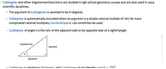
のCotDegreesは,直角三角形の隣辺と対辺の比である. - CotDegreesは,恒等式
を解してSinDegreesおよびCosDegreesと関連がある. - 特別な引数の場合,CotDegreesは,自動的に厳密値を計算する.
- CotDegreesは任意の数値精度で評価できる.
- CotDegreesは自動的にリストに縫い込まれる.
- CotDegreesは,Interval,CenteredInterval,Aroundの各オブジェクトに使うことができる.
- 記号操作・数値操作の両方に適した数学関数である.
例題
すべて開く すべて閉じる例 (6)
CotDegrees[60]単位辺を持つ直角三角形について45DegreeのCotDegreesを計算する:
Cot45deg = (1/1)Cot45deg == CotDegrees[45]Solve[CotDegrees[x] == Sqrt[3] && 0 < x < 90, x]Reduce[CotDegrees[x] > Sqrt[3] && 0 <= x <= 180, x]Plot[CotDegrees[x], {x, -180, 180}]Series[CotDegrees[x], {x, 0, 5}]スコープ (46)
数値評価 (6)
CotDegrees[1.2]N[CotDegrees[122 / 10], 50]CotDegrees[12.20000000000000000000000]CotDegreesは複素数入力を取ることができる:
CotDegrees[2.5 + I]CotDegreesを高精度で効率的に評価する:
CotDegrees[12.2`500]//TimingCotDegrees[12.2`100000];//TimingIntervalオブジェクトとCenteredIntervalオブジェクトを使って最悪の場合に保証される区間を計算する:
CotDegrees[Interval[{-45, 45}]]CotDegrees[CenteredInterval[60, 1 / 100]]CotDegrees[CenteredInterval[120 + 3I, (1 + I) / 100]]Aroundを使って平均的な場合の統計的区間を計算することもできる:
CotDegrees[Around[30, 0.01]]CotDegrees[{{60, 180}, {30, -90}}]MatrixFunctionを使って行列のCotDegrees関数を計算することもできる:
MatrixFunction[CotDegrees[#]&, {{60, 180}, {30, -90}}]特定の値 (6)
固定点におけるCotDegreesの値:
CotDegrees[{15, 30, 45, 60, 90, 180}]CotDegreesは,60度の有理倍で厳密値を持つ:
Table[CotDegrees[30n], {n, 1, 5}]CotDegrees[Infinity]CotDegrees[ComplexInfinity]CotDegrees[30]より複雑な場合はFunctionExpandを明示的に使う必要がある:
CotDegrees[180 / 8]FunctionExpand[%]CotDegreesの零点:
Assuming[m∈Integers, Refine[CotDegrees[180((1/2) + m)]]]Solveを使って1つの零点を求める:
sol = Solve[CotDegrees[x] == 0 && 0 < x < 180, x]xzero = x /. First[sol]Plot[CotDegrees[x], {x, 0, 180}, Rule[...]]CotDegreesの特異点:
Assuming[m∈Integers, FullSimplify[Refine[CotDegrees[180 m]]]]可視化 (4)
CotDegrees関数をプロットする:
Plot[CotDegrees[x], {x, -180, 180}]ComplexPlot3D[CotDegrees[z], {z, -180 - 100I, 180 + 100I}, Rule[...]]CotDegreesの実部をプロットする:
ComplexContourPlot[Re[CotDegrees[z]], {z, -180 - 60I, 180 + 60I}, ...]CotDegreesの虚部をプロットする:
ComplexContourPlot[Im[CotDegrees[z]], {z, -180 - 60I, 180 + 60I}, ...]CotDegreesの極プロット:
Table[PolarPlot[CotDegrees[k ϕ * 180 / π], {ϕ, 0, 2π}, ...], {k, 1, 4}]関数の特性 (13)
CotDegreesは周期が
の周期関数である:
CotDegrees[30] == CotDegrees[30 + 180]FunctionPeriodでこれを確認する:
FunctionPeriod[CotDegrees[x], x]CotDegreesの実領域:
FunctionDomain[CotDegrees[x], x]FunctionDomain[CotDegrees[z], z, Complexes]CotDegreesはすべての実数値に到達する:
FunctionRange[CotDegrees[x], x, y]FunctionRange[CotDegrees[x], x, y, Complexes]CotDegreesは偶関数である:
CotDegrees[-x]CotDegreesは鏡面特性
を有する:
FullSimplify[CotDegrees[Conjugate[z]] == Conjugate[CotDegrees[z]]]CotDegreesは解析関数ではない:
FunctionAnalytic[CotDegrees[x], x]FunctionMeromorphic[CotDegrees[x], x]CotDegreesは特定の範囲で単調である:
FunctionMonotonicity[CotDegrees[x], x]FunctionMonotonicity[{CotDegrees[x], 0 < x < 90}, x]CotDegreesは単射ではない:
FunctionInjective[CotDegrees[x], x]Plot[{CotDegrees[x], 1}, {x, -360, 360}]CotDegreesは全射である:
FunctionSurjective[CotDegrees[x], x]Plot[{CotDegrees[x], 20}, {x, -360, 360}]CotDegreesは非負でも非正でもない:
FunctionSign[CotDegrees[x], x]CotDegreesは180の倍数の点で特異点と不連続点を持つ:
FunctionSingularities[CotDegrees[x], x]FunctionDiscontinuities[CotDegrees[x], x]CotDegreesは凸でも凹でもない:
FunctionConvexity[CotDegrees[x], x]CotDegreesは,x が[0,90]のときは凸である:
FunctionConvexity[{CotDegrees[x], 0 < x < 90}, x]Plot[CotDegrees[x], {x, 0, 90}]TraditionalFormによる表示:
CotDegrees[α]//TraditionalForm微分 (3)
積分 (3)
Integrateを介してCotDegreesの不定積分を計算する:
Integrate[CotDegrees[x], x]Integrate[CotDegrees[ArcTanDegrees[z]], z]周期上のCotDegreesの定積分は0である:
Integrate[CotDegrees[x], {x, -90, 90}, PrincipalValue -> True]Integrate[CotDegrees[x]SinDegrees[x], x]Integrate[CotDegrees[z]^a, z]級数展開 (3)
Seriesを使ってテイラー(Taylor)展開を求める:
Series[CotDegrees[x], {x, 90, 7}]
の周囲のCotDegreesの最初の3つの近似をプロットする:
terms = Normal@Table[Series[CotDegrees[x], {x, 90, m}], {m, 0, 5, 2}];
Plot[{CotDegrees[x], terms}, {x, 0, 180}, PlotRange -> {{-5, 5}}]Series[CotDegrees[x], {x, 180, 5}]CotDegreesはベキ級数に適用できる:
CotDegrees[90 + x + (x^2/2) + (x^3/3) + O[x]^4]関数の恒等式と簡約 (5)
TrigExpandを使った倍角の公式:
TrigExpand[CotDegrees[2x]]TrigExpand[CotDegrees[x + y]]TrigExpand[CotDegrees[4x]]TrigReduceを使ってもとの式を回復する:
TrigReduce[%]TrigFactorを使って和を積に変換する:
TrigFactor[CotDegrees[x] + CotDegrees[y]]TrigToExpを使って指数関数に変換する:
TrigToExp[CotDegrees[z]]関数表現 (3)
TanDegreesを介した表現:
TanDegrees[90 - x]SinDegreesとCosDegreesを介した表現:
Simplify[CosDegrees[x] / SinDegrees[x]]SecDegreesとCscDegreesを介した表現:
Simplify[CscDegrees[x] / SecDegrees[x]]アプリケーション (12)
基本的な三角関数のアプリケーション (2)
のとき,恒等式
を使って角
のCotDegreesを求める:
Solve[x == (Sqrt[1 - y^2]/y) /. y -> (Sqrt[5]/3), x]Solve[CotDegrees[30] == x / 5, x]三角関数の恒等式 (4)
105度のCotDegreesの値を和と差の式を使って計算する:
CotDegrees[α + β]//TrigExpand% /. {α -> 60, β -> 45}//Simplify% == CotDegrees[105]15度のCotDegreesの値を半角の公式
を使って計算する:
(±Sqrt[(1 + CosDegrees[α]/1 - CosDegrees[α])] /. α -> 30)//Simplifyこの結果をCotDegreesを直接計算したものと比較する:
%[[1]] == CotDegrees[15]//NSimplify[CotDegrees[x] * (1 + SinDegrees[x])]Simplify[SinDegrees[x]CosDegrees[x] / CotDegrees[x] - 1]Simplify[CotDegrees[x]^2 * (1 - CosDegrees[x]^2) == (1 + CosDegrees[2x]/2)]三角関数の方程式 (2)
三角関数の不等式 (2)
より高度なアプリケーション (2)
Plot3D[Re[CotDegrees[x + I y]], {x, -180, 180}, {y, 0, 180}]CotDegrees関数の加法定理:
CotDegrees[ArcCotDegrees[x] + ArcCotDegrees[y]]//TrigExpand//Simplify特性と関係 (13)
CotDegrees[60] == Cot[π / 3]余接関数の基本的な偶奇性と周期性の特性は自動的に適用される:
CotDegrees[x + 180]CotDegrees[-x]CotDegrees[I x]1 / CotDegrees[x]//SimplifyCotDegrees[-x + 180k]Simplify[%, k∈Integers](CosDegrees[x]^2 - SinDegrees[x]^2/2 CosDegrees[x] SinDegrees[x])Simplify[%]FunctionExpandを使ってCotDegreesを根号によって表す:
{CotDegrees[180 / 8], CotDegrees[180 / 12], CotDegrees[180 / 15]}FunctionExpand[%]//Simplify{CotDegrees[ArcCotDegrees[z]], CotDegrees[2ArcCotDegrees[z]], CotDegrees[3ArcCotDegrees[z]]}FunctionExpand[%]//TogetherReduce[CotDegrees[z]^2 - 2CotDegrees[z + 45] == 4, z]FindRoot[CotDegrees[z]^2 + CotDegrees[z + 15] == 2, {z, 15, 150}]Plot[CotDegrees[z]^2 + CotDegrees[z + 15] - 2, {z, 15, 150}]CotDegreesの零点:
Reduce[CotDegrees[α x + β] == 0, x]CotDegreesの極:
Reduce[1 / CotDegrees[α x + β] == 0, x]Table[Residue[CotDegrees[z]^k, {z, 0}], {k, 10}](1/2π I)NIntegrate[CotDegrees[z], {z, -(1/4), -(I/4), +(1/4), +(I/4), -(1/4)}]FunctionExpandをCotDegreesに適用すると,三角関数の式がラジアン単位で生成される:
FunctionExpand[CotDegrees[x]]FunctionExpand[CotDegrees[x ^ 2]CotDegrees[120 - x / 2]]TrigToExpの出力にExpToTrigを適用すると三角関数がラジアン単位で生成される:
TrigToExp[CotDegrees[z]]ExpToTrig[%]TrigToExp[CotDegrees[2z]CotDegrees[z]];
ExpToTrig[%]CotDegreesは数値関数である:
NumericQ[CotDegrees[2 + E]]考えられる問題 (1)
おもしろい例題 (4)
Trigfunclist = {SinDegrees[θ], CosDegrees[θ], TanDegrees[θ], CotDegrees[θ], SecDegrees[θ], CscDegrees[θ]};
ratioslist = {a / c, b / c, a / b, b / a, c / b, c / a};Grid[...]//TraditionalFormSolve[CotDegrees[x] == SinDegrees[2x], x]//SimplifyReduce[CotDegrees[x] == SinDegrees[2x] && 0 < x < 90, x]//SimplifyCotDegrees[(180/2^12)]//FunctionExpand∫CotDegrees[x]^nⅆx関連するガイド
-
▪
- 三角関数
テキスト
Wolfram Research (2024), CotDegrees, Wolfram言語関数, https://reference.wolfram.com/language/ref/CotDegrees.html.
CMS
Wolfram Language. 2024. "CotDegrees." Wolfram Language & System Documentation Center. Wolfram Research. https://reference.wolfram.com/language/ref/CotDegrees.html.
APA
Wolfram Language. (2024). CotDegrees. Wolfram Language & System Documentation Center. Retrieved from https://reference.wolfram.com/language/ref/CotDegrees.html
BibTeX
@misc{reference.wolfram_2026_cotdegrees, author="Wolfram Research", title="{CotDegrees}", year="2024", howpublished="\url{https://reference.wolfram.com/language/ref/CotDegrees.html}", note=[Accessed: 15-September-2026]}
BibLaTeX
@online{reference.wolfram_2026_cotdegrees, organization={Wolfram Research}, title={CotDegrees}, year={2024}, url={https://reference.wolfram.com/language/ref/CotDegrees.html}, note=[Accessed: 15-September-2026]}