CotDegrees[θ]
给出了
度的余切.
CotDegrees
CotDegrees[θ]
给出了
度的余切.
更多信息
- CotDegrees 和其他三角函数是在高中几何课程中学习的内容,在许多科学学科中也有应用.
- CotDegrees 的参数单位假定为度.
- 当参数是
的简单有理倍数时,CotDegrees 会自动求值;对于更复杂的有理倍数,有时可以使用 FunctionExpand. - 角
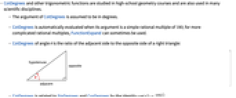
的 CotDegrees 是直角三角形的邻边与对边之比: - CotDegrees 和 SinDegrees 与 CosDegrees 的关系有恒等式
. - 对于某些特殊参数,CotDegrees 会自动求出精确值.
- CotDegrees 可以按照任意数值精度进行计算.
- CotDegrees 自动线性作用于列表.
- CotDegrees 可用于 Interval、CenteredInterval 和 Around 对象.
- 数学函数,适用于符号和数字运算.
范例
打开所有单元 关闭所有单元基本范例 (6)
CotDegrees[60]计算有单位边的直角三角形的 45 Degree 角的 CotDegrees:
Cot45deg = (1/1)Cot45deg == CotDegrees[45]Solve[CotDegrees[x] == Sqrt[3] && 0 < x < 90, x]Reduce[CotDegrees[x] > Sqrt[3] && 0 <= x <= 180, x]Plot[CotDegrees[x], {x, -180, 180}]Series[CotDegrees[x], {x, 0, 5}]范围 (46)
数值运算 (6)
CotDegrees[1.2]N[CotDegrees[122 / 10], 50]CotDegrees[12.20000000000000000000000]CotDegrees 可以接受复数输入:
CotDegrees[2.5 + I]高精度高效运算 CotDegrees:
CotDegrees[12.2`500]//TimingCotDegrees[12.2`100000];//Timing使用 Interval 和 CenteredInterval 对象计算最坏情况下的保证区间:
CotDegrees[Interval[{-45, 45}]]CotDegrees[CenteredInterval[60, 1 / 100]]CotDegrees[CenteredInterval[120 + 3I, (1 + I) / 100]]或者使用 Around 计算平均情况统计区间:
CotDegrees[Around[30, 0.01]]CotDegrees[{{60, 180}, {30, -90}}]或使用 MatrixFunction 计算矩阵 CotDegrees 函数:
MatrixFunction[CotDegrees[#]&, {{60, 180}, {30, -90}}]指定值 (6)
固定点的 CotDegrees 值:
CotDegrees[{15, 30, 45, 60, 90, 180}]CotDegrees 在 60 度的有理倍数处有精确值:
Table[CotDegrees[30n], {n, 1, 5}]CotDegrees[Infinity]CotDegrees[ComplexInfinity]CotDegrees[30]更复杂的情况需要明确使用 FunctionExpand:
CotDegrees[180 / 8]FunctionExpand[%]CotDegrees 的零点:
Assuming[m∈Integers, Refine[CotDegrees[180((1/2) + m)]]]使用 Solve 求解零点:
sol = Solve[CotDegrees[x] == 0 && 0 < x < 180, x]xzero = x /. First[sol]Plot[CotDegrees[x], {x, 0, 180}, Rule[...]]CotDegrees 的奇点:
Assuming[m∈Integers, FullSimplify[Refine[CotDegrees[180 m]]]]可视化 (4)
绘制 CotDegrees 函数:
Plot[CotDegrees[x], {x, -180, 180}]ComplexPlot3D[CotDegrees[z], {z, -180 - 100I, 180 + 100I}, Rule[...]]绘制 CotDegrees 的实部:
ComplexContourPlot[Re[CotDegrees[z]], {z, -180 - 60I, 180 + 60I}, ...]绘制 CotDegrees 的虚部:
ComplexContourPlot[Im[CotDegrees[z]], {z, -180 - 60I, 180 + 60I}, ...]使用 CotDegrees 绘制极坐标图:
Table[PolarPlot[CotDegrees[k ϕ * 180 / π], {ϕ, 0, 2π}, ...], {k, 1, 4}]函数属性 (13)
CotDegrees 是一个周期为
度的周期函数:
CotDegrees[30] == CotDegrees[30 + 180]用 FunctionPeriod 检验:
FunctionPeriod[CotDegrees[x], x]CotDegrees 的实值定义域:
FunctionDomain[CotDegrees[x], x]FunctionDomain[CotDegrees[z], z, Complexes]CotDegrees 可取所有实数值:
FunctionRange[CotDegrees[x], x, y]FunctionRange[CotDegrees[x], x, y, Complexes]CotDegrees 是奇函数:
CotDegrees[-x]CotDegrees 具有镜像属性
:
FullSimplify[CotDegrees[Conjugate[z]] == Conjugate[CotDegrees[z]]]CotDegrees 不是解析函数:
FunctionAnalytic[CotDegrees[x], x]FunctionMeromorphic[CotDegrees[x], x]CotDegrees 在特定范围内是单调函数:
FunctionMonotonicity[CotDegrees[x], x]FunctionMonotonicity[{CotDegrees[x], 0 < x < 90}, x]CotDegrees 不是单射函数:
FunctionInjective[CotDegrees[x], x]Plot[{CotDegrees[x], 1}, {x, -360, 360}]CotDegrees 是满射函数:
FunctionSurjective[CotDegrees[x], x]Plot[{CotDegrees[x], 20}, {x, -360, 360}]CotDegrees 既不是非负也不是非正:
FunctionSign[CotDegrees[x], x]CotDegrees 在 180 的倍数处既有奇点也有不连续点:
FunctionSingularities[CotDegrees[x], x]FunctionDiscontinuities[CotDegrees[x], x]CotDegrees 既不凸也不凹:
FunctionConvexity[CotDegrees[x], x]CotDegrees 对于区间 [0,90] 内的 x 为凸函数:
FunctionConvexity[{CotDegrees[x], 0 < x < 90}, x]Plot[CotDegrees[x], {x, 0, 90}]TraditionalForm 格式:
CotDegrees[α]//TraditionalForm微分 (3)
积分 (3)
通过 Integrate 计算 CotDegrees 的不定积分:
Integrate[CotDegrees[x], x]Integrate[CotDegrees[ArcTanDegrees[z]], z]一个周期内 CotDegrees 的定积分:
Integrate[CotDegrees[x], {x, -90, 90}, PrincipalValue -> True]Integrate[CotDegrees[x]SinDegrees[x], x]Integrate[CotDegrees[z]^a, z]级数展开 (3)
使用 Series 求泰勒展开式:
Series[CotDegrees[x], {x, 90, 7}]在
周围绘制 CotDegrees 前三个近似:
terms = Normal@Table[Series[CotDegrees[x], {x, 90, m}], {m, 0, 5, 2}];
Plot[{CotDegrees[x], terms}, {x, 0, 180}, PlotRange -> {{-5, 5}}]Series[CotDegrees[x], {x, 180, 5}]CotDegrees 可以应用于幂级数:
CotDegrees[90 + x + (x^2/2) + (x^3/3) + O[x]^4]函数恒等和化简 (5)
使用 TrigExpand 的双角公式:
TrigExpand[CotDegrees[2x]]TrigExpand[CotDegrees[x + y]]TrigExpand[CotDegrees[4x]]使用 TrigReduce 还原原始表达式:
TrigReduce[%]使用 TrigFactor 将和转换为积:
TrigFactor[CotDegrees[x] + CotDegrees[y]]使用 TrigToExp 转换为指数:
TrigToExp[CotDegrees[z]]函数表示 (3)
使用 TanDegrees 进行表示:
TanDegrees[90 - x]使用 SinDegrees 和 CosDegrees 进行表示:
Simplify[CosDegrees[x] / SinDegrees[x]]使用 SecDegrees 和 CscDegrees 进行表示:
Simplify[CscDegrees[x] / SecDegrees[x]]应用 (12)
基本三角函数应用 (2)
已知
,利用恒等式
求角
的 CotDegrees:
Solve[x == (Sqrt[1 - y^2]/y) /. y -> (Sqrt[5]/3), x]如果直角三角形的对边是 5,角是 30 度,求该直角三角形缺少的邻边长度:
Solve[CotDegrees[30] == x / 5, x]三角函数恒等式 (4)
使用和差公式计算 105 度的 CotDegrees 值:
CotDegrees[α + β]//TrigExpand% /. {α -> 60, β -> 45}//Simplify% == CotDegrees[105]使用半角公式
计算 15 度角的 CotDegrees 值:
(±Sqrt[(1 + CosDegrees[α]/1 - CosDegrees[α])] /. α -> 30)//Simplify将结果与直接计算的 CotDegrees 进行比较:
%[[1]] == CotDegrees[15]//NSimplify[CotDegrees[x] * (1 + SinDegrees[x])]Simplify[SinDegrees[x]CosDegrees[x] / CotDegrees[x] - 1]Simplify[CotDegrees[x]^2 * (1 - CosDegrees[x]^2) == (1 + CosDegrees[2x]/2)]三角方程 (2)
三角不等式 (2)
高级应用 (2)
Plot3D[Re[CotDegrees[x + I y]], {x, -180, 180}, {y, 0, 180}]CotDegrees 函数的加法定理:
CotDegrees[ArcCotDegrees[x] + ArcCotDegrees[y]]//TrigExpand//Simplify属性和关系 (13)
CotDegrees[60] == Cot[π / 3]CotDegrees[x + 180]CotDegrees[-x]CotDegrees[I x]1 / CotDegrees[x]//SimplifyCotDegrees[-x + 180k]Simplify[%, k∈Integers](CosDegrees[x]^2 - SinDegrees[x]^2/2 CosDegrees[x] SinDegrees[x])Simplify[%]使用 FunctionExpand 可用根式表示 CotDegrees:
{CotDegrees[180 / 8], CotDegrees[180 / 12], CotDegrees[180 / 15]}FunctionExpand[%]//Simplify{CotDegrees[ArcCotDegrees[z]], CotDegrees[2ArcCotDegrees[z]], CotDegrees[3ArcCotDegrees[z]]}FunctionExpand[%]//TogetherReduce[CotDegrees[z]^2 - 2CotDegrees[z + 45] == 4, z]FindRoot[CotDegrees[z]^2 + CotDegrees[z + 15] == 2, {z, 15, 150}]Plot[CotDegrees[z]^2 + CotDegrees[z + 15] - 2, {z, 15, 150}]CotDegrees 的零点:
Reduce[CotDegrees[α x + β] == 0, x]CotDegrees 的极点:
Reduce[1 / CotDegrees[α x + β] == 0, x]Table[Residue[CotDegrees[z]^k, {z, 0}], {k, 10}](1/2π I)NIntegrate[CotDegrees[z], {z, -(1/4), -(I/4), +(1/4), +(I/4), -(1/4)}]FunctionExpand 应用于 CotDegrees 会生成以弧度为单位的三角函数表达式:
FunctionExpand[CotDegrees[x]]FunctionExpand[CotDegrees[x ^ 2]CotDegrees[120 - x / 2]]ExpToTrig 应用于 TrigToExp 的输出将生成以弧度为单位的三角函数:
TrigToExp[CotDegrees[z]]ExpToTrig[%]TrigToExp[CotDegrees[2z]CotDegrees[z]];
ExpToTrig[%]CotDegrees 是一个数值函数:
NumericQ[CotDegrees[2 + E]]可能存在的问题 (1)
巧妙范例 (4)
Trigfunclist = {SinDegrees[θ], CosDegrees[θ], TanDegrees[θ], CotDegrees[θ], SecDegrees[θ], CscDegrees[θ]};
ratioslist = {a / c, b / c, a / b, b / a, c / b, c / a};Grid[...]//TraditionalFormSolve[CotDegrees[x] == SinDegrees[2x], x]//SimplifyReduce[CotDegrees[x] == SinDegrees[2x] && 0 < x < 90, x]//SimplifyCotDegrees[(180/2^12)]//FunctionExpand∫CotDegrees[x]^nⅆx相关指南
-
▪
- 三角函数
文本
Wolfram Research (2024),CotDegrees,Wolfram 语言函数,https://reference.wolfram.com/language/ref/CotDegrees.html.
CMS
Wolfram 语言. 2024. "CotDegrees." Wolfram 语言与系统参考资料中心. Wolfram Research. https://reference.wolfram.com/language/ref/CotDegrees.html.
APA
Wolfram 语言. (2024). CotDegrees. Wolfram 语言与系统参考资料中心. 追溯自 https://reference.wolfram.com/language/ref/CotDegrees.html 年
BibTeX
@misc{reference.wolfram_2026_cotdegrees, author="Wolfram Research", title="{CotDegrees}", year="2024", howpublished="\url{https://reference.wolfram.com/language/ref/CotDegrees.html}", note=[Accessed: 13-September-2026]}
BibLaTeX
@online{reference.wolfram_2026_cotdegrees, organization={Wolfram Research}, title={CotDegrees}, year={2024}, url={https://reference.wolfram.com/language/ref/CotDegrees.html}, note=[Accessed: 13-September-2026]}