CoxIngersollRossProcess[μ,σ,θ,x0]
長期平均μ,ボラティリティ σ,調整速度θ,初期条件 x0のCox–Ingersoll–Ross過程を表す.
CoxIngersollRossProcess

CoxIngersollRossProcess[μ,σ,θ,x0]
長期平均μ,ボラティリティ σ,調整速度θ,初期条件 x0のCox–Ingersoll–Ross過程を表す.
詳細
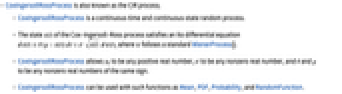
- CoxIngersollRossProcessはCIR過程としても知られている.
- CoxIngersollRossProcessは,連続時間・連続状態のランダム過程である.
- Cox–Ingersoll–Ross過程の状態
は伊藤微分方程式
を満たす.ただし,
は標準WienerProcess[]に従う. - CoxIngersollRossProcessでは,x0は任意の正の実数.σ は任意の非零の実数,θ および μ は同じ符号の任意の非零の実数でよい.
- CoxIngersollRossProcessは,Mean,PDF,Probability,RandomFunction等の関数で使うことができる.
例題
すべて開く すべて閉じる例 (3)
Cox–Ingersoll–Ross過程のシミュレーションを行う:
data = RandomFunction[CoxIngersollRossProcess[.3, .5, 1, 2], {0, 1, 0.01}]ListLinePlot[data, Filling -> Axis]Mean[CoxIngersollRossProcess[μ, σ, θ, Subscript[x, 0]][t]]Variance[CoxIngersollRossProcess[μ, σ, θ, Subscript[x, 0]][t]]CovarianceFunction[CoxIngersollRossProcess[μ, σ, θ, Subscript[x, 0]], s, t]Plot3D[CovarianceFunction[CoxIngersollRossProcess[.3, .5, 1, 2], s, t], {s, 0, 5}, {t, 0, 5}, ColorFunction -> "Rainbow"]スコープ (14)
基本的な用法 (9)
Cox–Ingersoll–Ross過程のランダムな経路の集合のシミュレーションを行う:
data = RandomFunction[CoxIngersollRossProcess[.3, .5, 1, 2], {0, 1, 0.01}, 3]ListLinePlot[data, Filling -> Axis]RandomFunction[CoxIngersollRossProcess[1 / 10, 1 / 3, 1, 2], {0, 1, 1 / 4}, WorkingPrecision -> 20]["Path"]sample[μ_] := (SeedRandom[14];RandomFunction[CoxIngersollRossProcess[μ, .3, .4, 1], {0, 1, .01}])ListStepPlot[sample[#], Filling -> Axis, PlotLabel -> StringJoin["μ = ", ToString[#]]]& /@ {.3, 1, 2}sample[σ_] := (SeedRandom[1];RandomFunction[CoxIngersollRossProcess[.5, σ, .4, 1], {0, 1, .01}])ListStepPlot[sample[#], Filling -> Axis, PlotLabel -> StringJoin["σ = ", ToString[#]]]& /@ {-1, 0.2, 1}sample[θ_] := (SeedRandom[1];RandomFunction[CoxIngersollRossProcess[.5, 1, θ, 1], {0, 1, .01}])ListStepPlot[sample[#], Filling -> Axis, PlotLabel -> StringJoin["θ = ", ToString[#]]]& /@ {0.2, 1, 4}さまざまな始点について,Cox–Ingersoll–Ross過程のシミュレーションを行う:
proc[x_] := CoxIngersollRossProcess[1, .4, .3, x];pts = {.5, 1, 3};SeedRandom[2];
ListLinePlot[RandomFunction[proc[#], {0, 10, .01}]& /@ pts, Filling -> Axis, PlotLegends -> (StringJoin["x = ", ToString[#]]& /@ pts)]data = RandomFunction[CoxIngersollRossProcess[.3, .5, 1, 2], {0, 100, 0.01}];EstimatedProcess[data, CoxIngersollRossProcess[μ, σ, θ, Subscript[x, 0]]]CorrelationFunction[CoxIngersollRossProcess[μ, σ, θ, Subscript[x, 0]], s, t]AbsoluteCorrelationFunction[CoxIngersollRossProcess[μ, σ, θ, Subscript[x, 0]], s, t]過程スライス特性 (5)
proc = CoxIngersollRossProcess[.3, .5, 1, 2];times = {.5, 1, 2};Plot[Evaluate@Table[PDF[proc[t], x], {t, times}], {x, 0, 3}, Filling -> Axis, PlotLegends -> {StringJoin["t = ", ToString[#]]& /@ times}]PDF[CoxIngersollRossProcess[μ, σ, θ, Subscript[x, 0]][t], x]Plot3D[PDF[CoxIngersollRossProcess[-.9, 1.2, -2.1, 3][{1, 2}], {x, y}], {x, 0, 10}, {y, 0, 15}]PDF[CoxIngersollRossProcess[μ, σ, θ, Subscript[x, 0]][{1, 2}], {x, y}]Expectation[x[t] ^ 2, xCoxIngersollRossProcess[μ, σ, θ, Subscript[x, 0]]]Probability[x[t] < 6, xCoxIngersollRossProcess[μ, σ, θ, Subscript[x, 0]]]Skewness[CoxIngersollRossProcess[μ, σ, θ, Subscript[x, 0]][t]]//Simplify[#, σ > 0]&Kurtosis[CoxIngersollRossProcess[μ, σ, θ, Subscript[x, 0]][t]]//SimplifyMoment[CoxIngersollRossProcess[μ, σ, θ, Subscript[x, 0]][t], r]CharacteristicFunction[CoxIngersollRossProcess[μ, σ, θ, Subscript[x, 0]][t], w]MomentGeneratingFunction[CoxIngersollRossProcess[μ, σ, θ, Subscript[x, 0]][t], w]CentralMomentおよびその母関数:
CentralMoment[CoxIngersollRossProcess[μ, σ, θ, Subscript[x, 0]][t], 2]CentralMomentGeneratingFunction[CoxIngersollRossProcess[μ, σ, θ, Subscript[x, 0]][t], w]FactorialMomentおよびその母関数:
FactorialMoment[CoxIngersollRossProcess[μ, σ, θ, Subscript[x, 0]][t], 2]FactorialMomentGeneratingFunction[CoxIngersollRossProcess[μ, σ, θ, Subscript[x, 0]][t], w]Cumulantおよびその母関数:
Cumulant[CoxIngersollRossProcess[μ, σ, θ, Subscript[x, 0]][t], r]CumulantGeneratingFunction[CoxIngersollRossProcess[μ, σ, θ, Subscript[x, 0]][t], w]特性と関係 (3)
WeakStationarity[CoxIngersollRossProcess[μ, σ, θ, Subscript[x, 0]]]Table[Plot[NProbability[(x[5] <= Subscript[x, 2])(x[2] == Subscript[x, 1]), xCoxIngersollRossProcess[.3, 1, .3, 1.2]], {Subscript[x, 2], 0, 6}, Filling -> Axis, PlotLabel -> Row[{"SubscriptBox[x, 1] = ", Subscript[x, 1]}]], {Subscript[x, 1], {.3, 1, 2.3, 3}}]Cox–ingersoll–Ross過程は特殊なItoProcessである:
ItoProcess[CoxIngersollRossProcess[μ, σ, θ, Subscript[x, 0]]]StratonovichProcessでもある:
StratonovichProcess[CoxIngersollRossProcess[μ, σ, θ, Subscript[x, 0]]]おもしろい例題 (3)
Cox–Ingersoll–Ross過程のシミュレーションを二次元で行う:
SeedRandom[103];sample = RandomFunction[CoxIngersollRossProcess[.3, .5, 1, 2], {0, 1, .001}, 2]["ValueList"];ListLinePlot[Transpose@sample, ColorFunction -> "FallColors"]Cox–Ingersoll–Ross過程のシミュレーションを三次元で行う:
proc = CoxIngersollRossProcess[-.4, .5, -1.3, 2];
SeedRandom[123];
sample = Table[RandomFunction[proc, {0, 1, 0.01}, 3]["ValueList"], {6}];Graphics3D@Table[{ColorData["SolarColors"][RandomReal[]], Tube@Line@sample[[i]]}, {i, 6}]Cox–Ingersoll–Ross過程から500経路のシミュレーションを行う:
data = RandomFunction[CoxIngersollRossProcess[.4, .5, .3, 2], {0, 1, .01}, 500];sd = data["SliceData", 1];cf = ColorData["Rainbow"];
sliced = BarChart[Last[#], Axes -> False, BarOrigin -> Left, AspectRatio -> 4, ChartStyle -> (cf /@ Rescale[MovingAverage[First[#], 2], {Min[sd], Max[sd]}, {0, 1}]), ImageSize -> 62]&[HistogramList[sd, {Range[Min[sd], Max[sd], (Max[sd] - Min[sd]) / 20]}]];1におけるスライス分布の経路とヒストグラム分布をプロットする:
ListLinePlot[data, ImageSize -> 400, PlotRange -> All,
AspectRatio -> 3 / 4, Epilog -> Inset[sliced, {1.01, 2}, {0, 10}], PlotStyle -> (cf /@ Rescale[sd]), BaseStyle -> Directive[Thin, Opacity[0.5]], PlotRangePadding -> {{0, .25}, {.5, .5}}]関連するガイド
-
▪
- パラメトリック確率過程 ▪
- 確率微分方程式過程
テキスト
Wolfram Research (2012), CoxIngersollRossProcess, Wolfram言語関数, https://reference.wolfram.com/language/ref/CoxIngersollRossProcess.html.
CMS
Wolfram Language. 2012. "CoxIngersollRossProcess." Wolfram Language & System Documentation Center. Wolfram Research. https://reference.wolfram.com/language/ref/CoxIngersollRossProcess.html.
APA
Wolfram Language. (2012). CoxIngersollRossProcess. Wolfram Language & System Documentation Center. Retrieved from https://reference.wolfram.com/language/ref/CoxIngersollRossProcess.html
BibTeX
@misc{reference.wolfram_2026_coxingersollrossprocess, author="Wolfram Research", title="{CoxIngersollRossProcess}", year="2012", howpublished="\url{https://reference.wolfram.com/language/ref/CoxIngersollRossProcess.html}", note=[Accessed: 06-September-2026]}
BibLaTeX
@online{reference.wolfram_2026_coxingersollrossprocess, organization={Wolfram Research}, title={CoxIngersollRossProcess}, year={2012}, url={https://reference.wolfram.com/language/ref/CoxIngersollRossProcess.html}, note=[Accessed: 06-September-2026]}

