Wolfram 语言与系统参考资料中心

DFixedPoints

DFixedPoints[eqn,x[t],t]

给出微分方程的不动点.

DFixedPoints[{eqn₁,eqn₂,…},{x₁[t],x₂[t],…},t]

给出微分方程组的不动点.

范例

打开所有单元关闭所有单元

基本范例 (4)

求方程的不动点：

Wolfram Language code: DFixedPoints[x'[t] == -2x[t], x[t], t]

求方程的不动点：

Wolfram Language code: DFixedPoints[x'[t] == 2x[t] + 1, x[t], t]

求方程的不动点和稳定条件：

Wolfram Language code: DFixedPoints[y'[t] == a y[t], y, t]

Wolfram Language code: DStabilityConditions[y'[t] == a y[t], y, t]

绘制 a 的不同值的几个解：

Wolfram Language code: sol = DSolveValue[{y'[t] == a y[t], y[0] == -1}, y[t], t]

Wolfram Language code: Table[Plot[sol, {t, 0, 4}, Rule[...]], {a, {-1.1, 1.1}}]

二维系统的不动点和稳定性分析：

Wolfram Language code: DFixedPoints[{x'[t] == b x[t] + y[t], y'[t] == -2 x[t] + a y[t]}, {x, y}, t]

Wolfram Language code: DStabilityConditions[{x'[t] == b x[t] + y[t], y'[t] == -2 x[t] + a y[t]}, {x, y}, t]

绘制系统稳定的参数区域：

Wolfram Language code: RegionPlot[%[[1, 2]], {a, -5, 5}, {b, -5, 5}]

范围 (23)

线性方程 (5)

求方程的不动点：

Wolfram Language code: DFixedPoints[x'[t] == -3 x[t], x, t]

一阶线性非齐次方程：

Wolfram Language code: DFixedPoints[y'[t] == a y[t] + 5, y, t]

Wolfram Language code: DStabilityConditions[y'[t] == a y[t] + 5, y, t]

绘制时不稳定解的图形：

Wolfram Language code:

sol = DSolveValue[{y'[t] == a y[t] + 5, y[0] == 1}, y[t], t];
Plot[sol /. a -> 0.5, {t, 0, 10}]

绘制时稳定解的图形：

Wolfram Language code:

sol = DSolveValue[{y'[t] == a y[t] + 5, y[0] == 1}, y[t], t];
Plot[sol /. a -> -0.5, {t, 0, 10}]

二阶线性方程：

Wolfram Language code: DFixedPoints[y''[t] + a y'[t] + b y[t] == 0, y, t]

三阶线性方程：

Wolfram Language code: DFixedPoints[y'''[t] + a y''[t] + b y'[t] + c y[t] == 0, y, t]

高阶非齐次常微分方程：

Wolfram Language code: DFixedPoints[y'''[x] + 5y''[x] + 3y'[x] + 6y[x] == 3, y, x]

使用固定点的坐标作为初始值求解常微分方程：

Wolfram Language code: DSolve[{y'''[x] + 5y''[x] + 3y'[x] + 6y[x] == 3, y[0] == 1 / 2, y'[0] == 0, y''[0] == 0}, y[x], x]

非线性方程 (3)

非线性微分方程的稳定性分析：

Wolfram Language code: DFixedPoints[x'[t] == x[t]^2 + 3x[t], x, t]

Wolfram Language code: DStabilityConditions[x'[t] == x[t]^2 + 3x[t], x, t]

使用 StreamPlot 证明稳定性：

Wolfram Language code: StreamPlot[{1, x^2 + 3x}, {t, 0, 10}, {x, -4, 1}]

一阶非线性方程的稳定性：

Wolfram Language code: DFixedPoints[x'[t] == x[t]^2 - 5x[t] + 6, x, t]

Wolfram Language code: DStabilityConditions[x'[t] == x[t]^2 - 5x[t] + 6, x, t]

绘制初始值为时解的图形：

Wolfram Language code: sol = DSolveValue[{x'[t] == x[t]^2 - 5x[t] + 6, x[0] == 5 / 2}, x[t], t]

Wolfram Language code: Plot[sol, {t, 0, 10}, PlotRange -> All]

使用 StreamPlot 证明点处的稳定性：

Wolfram Language code: StreamPlot[{1, x^2 - 5x + 6}, {t, 0, 10}, {x, 0, 4}]

考虑二阶非线性常微分方程：

Wolfram Language code: eqn = y[x]^2 + 3 y'[x] + y''[x] == 2;

DSolve 无法解这个方程：

Wolfram Language code: DSolve[eqn, y, x]

使用 DFixedPoints 找到方程的不动点：

Wolfram Language code: DFixedPoints[eqn, y, x]

将方程转换为一阶常微分方程组：

Wolfram Language code: sys = {y'[x] == y1[x], y[x]^2 + 3 y1[x] + y1'[x] == 2};

在平面绘制系统的轨迹：

Wolfram Language code: StreamPlot[{y1, 2 - y^2 - 3y1}, {y, -3, 3}, {y1, -3, 3}, ...]

线性系统 (11)

稳定的线性非耦合方程组：

Wolfram Language code: DFixedPoints[{x'[t] == -x[t], y'[t] == -y[t]}, {x, y}, t]

系统轨迹：

Wolfram Language code: StreamPlot[{-x, -y}, {x, -3, 3}, {y, -3, 3}, ...]

不稳定的线性非耦合方程组：

Wolfram Language code: DFixedPoints[{x'[t] == x[t], y'[t] == y[t]}, {x, y}, t]

系统轨迹：

Wolfram Language code: StreamPlot[{x, y}, {x, -3, 3}, {y, -3, 3}, ...]

具有常数系数的线性系统的稳定性：

Wolfram Language code: DFixedPoints[{x'[t] == -x[t] - y[t], y'[t] == 2x[t] - y[t]}, {x, y}, t]

Wolfram Language code: DStabilityConditions[{x'[t] == -x[t] - y[t], y'[t] == 2x[t] - y[t]}, {x, y}, t]

使用 StreamPlot 来可视化稳定性：

Wolfram Language code:

StreamPlot[{-x - y, 2x - y}, {x, -3, 3}, {y, -3, 3}, StreamPoints -> Coarse, Epilog -> {Red, PointSize[Medium], Point[{0, 0}]}]

具有常数系数的不稳定系统：

Wolfram Language code: DFixedPoints[{x'[t] == 3x[t] - 4y[t], y'[t] == x[t] - y[t]}, {x, y}, t]

系统轨迹：

Wolfram Language code: StreamPlot[{3x - 4y, x - y}, {x, -3, 3}, {y, -3, 3}, Rule[...]]

具有常数系数的稳定系统：

Wolfram Language code: DFixedPoints[{x'[t] == -y[t], y'[t] == x[t]}, {x, y}, t]

系统轨迹：

Wolfram Language code: StreamPlot[{-y, x}, {x, -3, 3}, {y, -3, 3}, Rule[...]]

非齐次不稳定系统：

Wolfram Language code: DFixedPoints[{x'[t] == x[t] + y[t] - 2, y'[t] == x[t] - y[t]}, {x, y}, t]

系统轨迹：

Wolfram Language code: StreamPlot[{x + y - 2, x - y}, {x, -3, 3}, {y, -3, 3}, Rule[...]]

非齐次稳定系统：

Wolfram Language code: DFixedPoints[{x'[t] == -x[t] - y[t] - 1, y'[t] == 2x[t] - y[t] + 5}, {x, y}, t]

Wolfram Language code: StreamPlot[{-x - y - 1, 2x - y + 5}, {x, -3, 3}, {y, -3, 3}, Rule[...]]

绘制解的图形：

Wolfram Language code: sol = DSolveValue[{x'[t] == -x[t] - y[t] - 1, y'[t] == 2x[t] - y[t] + 5, x[0] == 2, y[0] == 0}, {x[t], y[t]}, t]

Wolfram Language code: Plot[sol, {t, 0, 10}]

对于由两个二阶 ODE 组成的方程组，不动点是嵌套列表 {{y,y'},{z,z'}}：

Wolfram Language code: DFixedPoints[{-z[t] - 3 y'[t] + y''[t] == 2, z''[t] == y[t] + z'[t] - z[t] - 3}, {y, z}, t]

具有符号系数的线性系统：

Wolfram Language code: DFixedPoints[{x'[t] == β y[t] + α, y'[t] == δ x[t] - γ}, {x, y}, t]

由四个线性常微分方程组成的系统：

Wolfram Language code:

DFixedPoints[{Derivative[1][x][t] == 2 x[t] - 5 y[t], Derivative[1][y][t] == x[t] - 2 y[t], Derivative[1][u][t] == u[t] + 2 v[t], Derivative[1][v][t] == -5 u[t] - v[t]}, {x, y, u, v}, t]

绘制解的图形：

Wolfram Language code:

sol = DSolveValue[{Derivative[1][x][t] == 2 x[t] - 5 y[t], Derivative[1][y][t] == x[t] - 2 y[t], Derivative[1][u][t] == u[t] + 2 v[t], Derivative[1][v][t] == -5 u[t] - v[t]}, {x[t], y[t], u[t], v[t]}, t]

Wolfram Language code: Plot[Evaluate[sol /. {C[1] -> 1, C[2] -> 2, C[3] -> 3, C[4] -> 4}], {t, 0, 10}]

具有随机常数系数的 10×10 线性系统：

Wolfram Language code:

SeedRandom[1234];
m = RandomInteger[10, {10, 10}];
g = RandomInteger[10, 10];

Wolfram Language code: dep = {x1[t], x2[t], x3[t], x4[t], x5[t], x6[t], x7[t], x8[t], x9[t], x10[t]};

Wolfram Language code: sys = Thread[D[dep, t] == m.dep + g];

Wolfram Language code: DFixedPoints[sys, dep, t]

非线性系统 (4)

非线性一阶系统：

Wolfram Language code: DFixedPoints[{x'[t] == −x[t] + 2x[t] y[t], y'[t] == y[t]−x[t]^2−y[t]^2}, {x, y}, t]

分析各点的稳定性：

Wolfram Language code: DStabilityConditions[{x'[t] == −x[t] + 2x[t] y[t], y'[t] == y[t]−x[t]^2−y[t]^2}, {x, y}, t]

使用 StreamPlot 来可视化稳定性：

Wolfram Language code: StreamPlot[{−x + 2x y, y−x^2−y^2}, {x, -2, 2}, {y, -1, 2}, Rule[...]]

具有周期不动点的非线性系统：

Wolfram Language code: DFixedPoints[{x'[t] == y[t], y'[t] == Sin[x[t]]}, {x, y}, t]

分析各点的稳定性：

Wolfram Language code: DStabilityConditions[{x'[t] == y[t], y'[t] == Sin[x[t]]}, {x, y}, t]

Wolfram Language code: StreamPlot[{y, Sin[x]}, {x, -4Pi, 4Pi}, {y, -6, 6}, Rule[...]]

在原点处有不稳定不动点的非线性系统：

Wolfram Language code: DFixedPoints[{y[t] + x[t](1−x[t]^2−y[t]^2) == x'[t], −x[t] + y[t](1−x[t]^2−y[t]^2) == y'[t]}, {x, y}, t]

Wolfram Language code:

StreamPlot[{y + x(1−x^2−y^2), −x + y(1−x^2−y^2)}, {x, -3, 3}, {y, -3, 3}, Epilog -> {Blue, PointSize[Medium], Point[{0, 0}]}]

高阶非线性方程组：

Wolfram Language code: DFixedPoints[{x''[t] == -2(x[t]^2 + y[t]^2)x'[t] - x[t] - 1, y''[t] == -2(x[t]^2 + y[t]^2)y'[t] - y[t]}, {x, y}, t]

选项 (1)

Assumptions (1)

由两个非线性方程组成的方程组具有无数个周期不动点：、

Wolfram Language code: DFixedPoints[{x'[t] == y[t], y'[t] == Sin[x[t]]}, {x, y}, t]

使用 Assumptions 来指定因变量的范围：

Wolfram Language code: DFixedPoints[{x'[t] == y[t], y'[t] == Sin[x[t]]}, {x, y}, t, Assumptions -> -4 < x[t] < 4]

应用 (11)

物理学 (5)

带阻尼的弹簧质量系统的稳定性分析：

Wolfram Language code: DFixedPoints[m u''[t] + c u'[t] + k u[t] == 0, u, t]

Wolfram Language code: DStabilityConditions[m u''[t] + c u'[t] + k u[t] == 0, u, t]

利用假设简化稳定性条件：

Wolfram Language code: DStabilityConditions[m u''[t] + c u'[t] + k u[t] == 0, u, t, Assumptions -> m > 0 && c > 0 && k > 0]

求解弹簧质量系统方程：

Wolfram Language code: sol = DSolveValue[{m u''[t] + c u'[t] + k u[t] == 0, u[0] == 1, u'[0] == 0}, u[t], t]

绘制给定参数值时解的图形：

Wolfram Language code: Plot[sol /. {m -> 1, k -> 1, c -> 0.5}, {t, 0, 20}, PlotRange -> All]

对电路方程做稳定性分析：

Wolfram Language code: DFixedPoints[l i''[t] + r i'[t] + (1/c) i[t] == 0, i, t]

Wolfram Language code: DStabilityConditions[l i''[t] + r i'[t] + (1/c) i[t] == 0, i, t]

求解电路方程：

Wolfram Language code: sol = DSolveValue[{l i''[t] + r i'[t] + (1/c) i[t] == 0, i[0] == 1, i'[0] == 0}, i[t], t]

绘制给定参数值时解的图形：

Wolfram Language code: Plot[sol /. {r -> 0.1, l -> 5 10^-2, c -> 0.1}, {t, 0, 10}, PlotRange -> All]

阻尼摆方程的稳定性分析：

Wolfram Language code: DFixedPoints[θ''[t] + 1 / 5 θ'[t] + 9 Sin[θ[t]] == 0, θ, t]

Wolfram Language code: DStabilityConditions[θ''[t] + 1 / 5 θ'[t] + 9 Sin[θ[t]] == 0, θ, t]

绘制系统的相图：

Wolfram Language code: StreamPlot[{θ1, -1 / 5θ1 - 9Sin[θ]}, {θ, -3Pi, 3Pi}, {θ1, -10, 10}, ...]

绘制初始条件为 , 时解的图形：

Wolfram Language code:

sol = NDSolve[{θ''[t] + 1 / 5 θ'[t] + 9 Sin[θ[t]] == 0, θ[0] == Pi / 2, θ'[0] == 0}, θ[t], {t, 0, 20}];
Plot[θ[t] /. sol, {t, 0, 20}, PlotRange -> All]

稳定的洛伦兹方程组：

Wolfram Language code:

σ = 10;
b = 8 / 3;
r = 15;
eqns = {σ(−x[t] + y[t]) == x'[t], r x[t]−y[t]−x[t] z[t] == y'[t], −b z[t] + x[t] y[t] == z'[t]};

Wolfram Language code: DFixedPoints[eqns, {x, y, z}, t]

Wolfram Language code: DStabilityConditions[eqns, {x, y, z}, t]

使用 StreamPlot3D 可视化洛伦兹吸引子：

Wolfram Language code: StreamPlot3D[{σ(−x + y), r x−y−x z, −b z + x y}, {x, -10, 10}, {y, -10, 10}, {z, 0, 20}]

不稳定的洛伦兹方程组：

Wolfram Language code:

σ = 10;
b = 8 / 3;
r = 28;
eqns = {σ(−x[t] + y[t]) == x'[t], r x[t]−y[t]−x[t] z[t] == y'[t], −b z[t] + x[t] y[t] == z'[t]};

Wolfram Language code: DFixedPoints[eqns, {x, y, z}, t]

Wolfram Language code: DStabilityConditions[eqns, {x, y, z}, t]

求解方程组并绘制解的图形：

Wolfram Language code: sol = NDSolve[{eqns, x[0] == 10, y[0] == 10, z[0] == 20}, {x[t], y[t], z[t]}, {t, 0, 200}];

Wolfram Language code: ParametricPlot3D[{x[t], y[t], z[t]} /. sol, {t, 0, 200}, PlotPoints -> 200, ColorFunction -> (Hue[#4]&)]

生物 (3)

捕食者-猎物模型的稳定性分析（Lotka–Volterra 方程）：

Wolfram Language code: DFixedPoints[{x'[t] == x[t](1 - 1 / 2y[t]), y'[t] == y[t](-3 / 4 + 1 / 4x[t])}, {x, y}, t]

Wolfram Language code: DStabilityConditions[{x'[t] == x[t](1 - 1 / 2y[t]), y'[t] == y[t](-3 / 4 + 1 / 4x[t])}, {x, y}, t]

绘制系统的相图：

Wolfram Language code: StreamPlot[{x(1 - 1 / 2y), y(-3 / 4 + 1 / 4x)}, {x, 0, 8}, {y, 0, 4}, Rule[...]]

求解初始条件为、的系统：

Wolfram Language code:

sol = NDSolve[{x'[t] == x[t](1 - 1 / 2y[t]), y'[t] == y[t](-3 / 4 + 1 / 4x[t]), x[0] == 2, y[0] == 1}, {x[t], y[t]}, {t, 0, 30}]

绘制解的图形：

Wolfram Language code: Plot[Evaluate[{x[t], y[t]} /. sol], {t, 0, 30}, PlotLegends -> {"Prey", "Predator"}, PlotRange -> {0, 7}]

罗森茲威格-麦克阿瑟（Rosenzweig-MacArthur ）捕食者-猎物模型：

Wolfram Language code: eqns = {n'[t] == n[t](1 - n[t] / k) - an p[t]n[t] / (n[t] + h), p'[t] == p[t](ap n[t] / (n[t] + h) - m)};

Wolfram Language code: params = {an -> 1, ap -> 2, h -> 1, m -> 1, k -> 4};

Wolfram Language code: DFixedPoints[eqns /. params, {n, p}, t]

Wolfram Language code: StreamPlot[{n(1 - n / k) - an p n / (n + h), p(ap n / (n + h) - m)} /. params, {n, 0, 4}, {p, 0, 4}, Rule[...]]

恒化器（chemostat）模型代表微生物在非生物资源上生长的生物系统：

Wolfram Language code: model = {x'[t] == (k x[t]y[t]/1 + y[t]) - x[t], y'[t] == -(x[t]y[t]/1 + y[t]) - y[t] + q};

找到不动点：

Wolfram Language code: DFixedPoints[model, {x, y}, t]//Simplify

分析和时模型的稳定性：

Wolfram Language code: DStabilityConditions[model /. {k -> 2, q -> 2}, {x, y}, t]

Wolfram Language code: StreamPlot[{(k x y/1 + y) - x, -(x y/1 + y) - y + q} /. {k -> 2, q -> 2}, {x, 0, 4}, {y, 0, 3}, Rule[...]]

化学 (1)

Brusselator 是一种自催化反应的理论模型. Brusselator 模型的速率方程为：

Wolfram Language code: sys = {x'[t] == x[t]^2y[t] - (b + 1)x[t] + a, y'[t] == -x[t]^2y[t] + b x[t]};

求系统的不动点：

Wolfram Language code: DFixedPoints[sys, {x, y}, t]

如果 b<1+a²，则该点是稳定的：

Wolfram Language code: DStabilityConditions[sys /. {a -> 1, b -> 3 / 2}, {x, y}, t]

Wolfram Language code: StreamPlot[{x^2y - (b + 1)x + a, -x^2y + b x} /. {a -> 1, b -> 3 / 2}, {x, 0, 3}, {y, 0, 4}, Rule[...]]

如果 b>1+a²，则该点不稳定：

Wolfram Language code: DStabilityConditions[sys /. {a -> 1, b -> 5 / 2}, {x, y}, t]

Wolfram Language code: StreamPlot[{x^2y - (b + 1)x + a, -x^2y + b x} /. {a -> 1, b -> 5 / 2}, {x, 0, 3}, {y, 0, 4}, Rule[...]]

控制系统 (2)

从欧拉运动方程开始分析卫星的姿态动力学：

具有主惯性矩 , , 的欧拉方程：

Wolfram Language code:

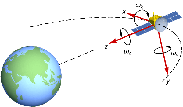
eqns = Table[Subscript[j, i[[1]]] Subscript[ω, i[[1]]]'[t] - (Subscript[j, i[[2]]] - Subscript[j, i[[3]]])Subscript[ω, i[[2]]][t]Subscript[ω, i[[3]]][t] == Subscript[τ, i[[1]]][t], {i, {{x, y, z}, {y, z, x}, {z, x, y}}}] /. {Subscript[j, x] -> 300, Subscript[j, y] -> 320, Subscript[j, z] -> 270}

对于 , , 的固定值，求方程的不动点：

Wolfram Language code:

DFixedPoints[eqns /. {Subscript[τ, x][t] -> -27 / 400, Subscript[τ, y][t] -> 3 / 200, Subscript[τ, z][t] -> 1 / 50}, {Subscript[ω, x], Subscript[ω, y], Subscript[ω, z]}, t]

选择不动点作为工作点：

Wolfram Language code:

opPt = {Subscript[ω, x0] -> (1/30Sqrt[3]), Subscript[ω, y0] -> (3Sqrt[3]/100), Subscript[ω, z0] -> (3Sqrt[3]/200), Subscript[τ, x0] -> -(27/400), Subscript[τ, y0] -> (3/200), Subscript[τ, z0] -> (1/50)};

构建状态空间模型：

Wolfram Language code:

ssm = StateSpaceModel[eqns, {{Subscript[ω, x][t], Subscript[ω, x0]}, {Subscript[ω, y][t], Subscript[ω, y0]}, {Subscript[ω, z][t], Subscript[ω, z0]}}, {{Subscript[τ, x][t], Subscript[τ, x0]}, {Subscript[τ, y][t], Subscript[τ, y0]}, {Subscript[τ, z][t], Subscript[τ, z0]}}, {Subscript[ω, x][t], Subscript[ω, y][t], Subscript[ω, z][t]}, t, SystemsModelLabels -> {{Subscript[τ, x], Subscript[τ, y], Subscript[τ, z]}, {Subscript[ω, x], Subscript[ω, y], Subscript[ω, z]}, {Subscript[ω, x], Subscript[ω, y], Subscript[ω, z]}}] /. opPt

卫星姿态如果受到干扰则不受控制：

Wolfram Language code:

OutputResponse[{ssm, {0.2, -0.1, 0.35}}, {0, 0, 0}, {t, 0, 3000}];
Plot[%, {t, 0, 3000}, PlotRange -> All, PlotLegends -> {Subscript[ω, x], Subscript[ω, y], Subscript[ω, z]}]

验证模型的可控性：

Wolfram Language code: ControllableModelQ[ssm]

使用拉格朗日法研究倒立摆：

的位置：

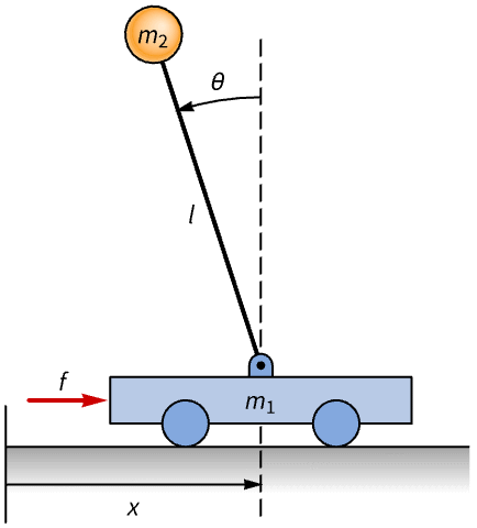
Wolfram Language code: Subscript[r, p] = Composition[TranslationTransform[{x[t], 0, 0}], RotationTransform[θ[t], {0, 0, 1}]][{0, 1, 0}]

其速度：

Wolfram Language code: Subscript[v, p] = D[Subscript[r, p], t]

小车和摆的动能：

Wolfram Language code: 𝒦 = (1/2)Subscript[m, 1] x'[t]^2 + (1/2)Subscript[m, 2]Subscript[v, p].Subscript[v, p]

摆的势能：

Wolfram Language code: 𝒰 = Subscript[m, 2]g Subscript[r, p][[2]]

拉格朗日量：

Wolfram Language code: ℒ = 𝒦 - 𝒰

广义的力：

Wolfram Language code: {Subscript[f, x], Subscript[f, θ]} = D[f[t] δx - Subscript[b, x]x'[t]δx - Subscript[b, θ]θ'[t]δθ, {{δx, δθ}}]

运动方程：

Wolfram Language code: eqns = Table[Subscript[∂, t]D[ℒ, q'[t]] - D[ℒ, q[t]] == Subscript[f, q], {q, {x, θ}}]//Simplify

状态空间模型：

Wolfram Language code:

ssm = StateSpaceModel[eqns, {x[t], x'[t], θ[t], θ'[t]}, f[t], {x[t], θ[t]}, t, SystemsModelLabels -> {f, {x, θ}, {x, Derivative[1][x], θ, Derivative[1][θ]}}]

非正特征值使其成为一个不稳定的系统：

Wolfram Language code:

Eigenvalues[First[Normal[ssm /. {Subscript[m, 1] -> 1 / 2, Subscript[m, 2] -> 1 / 10, l -> 3 / 10, g -> 10, Subscript[b, x] -> 15 / 100, Subscript[b, θ] -> 1 / 100}]]]//N

Wolfram Language code:

DFixedPoints[eqns /. {Subscript[m, 1] -> 1 / 2, Subscript[m, 2] -> 1 / 10, l -> 3 / 10, g -> 10, Subscript[b, x] -> 15 / 100, Subscript[b, θ] -> 1 / 100, f[t] -> 0}, {x, θ}, t]

Wolfram Language code:

DStabilityConditions[eqns /. {Subscript[m, 1] -> 1 / 2, Subscript[m, 2] -> 1 / 10, l -> 3 / 10, g -> 10, Subscript[b, x] -> 15 / 100, Subscript[b, θ] -> 1 / 100, f[t] -> 0}, {x, θ}, t, {{1, 0, 2Pi, 0}, {1, 0, 3Pi, 0}}]

属性和关系 (8)

DFixedPoints 返回微分方程的不动点：

Wolfram Language code: DFixedPoints[y'[t] == a y[t], y, t]

Wolfram Language code: DFixedPoints[y'[t] == (1/2)y[t] + 1, y, t]

使用 DFixedPoints 求微分方程的所有不动点：

Wolfram Language code: DFixedPoints[y'[t] == 2 y[t](1 - y[t]), y[t], t]

使用 DStabilityConditions 分析特定固定点的稳定性：

Wolfram Language code: DStabilityConditions[y'[t] == 2 y[t](1 - y[t]), y[t], t, {{0}}]

Wolfram Language code: DStabilityConditions[y'[t] == 2 y[t](1 - y[t]), y[t], t, {{1}}]

使用 DFixedPoints 求非线性常微分方程的所有不动点：

Wolfram Language code: points = DFixedPoints[x'[t] == x[t]^2 + 3x[t], x, t]

使用 Solve 求不动点：

Wolfram Language code: Solve[x^2 + 3x == 0, x]

n 阶微分方程的不动点是 n 维向量：

Wolfram Language code: DFixedPoints[y''[t] + y'[t] + 3 y[t] == 5, y, t]

由 n 个一阶微分方程组成的系统的不动点是 n 维向量：

Wolfram Language code: DFixedPoints[{y'[t] + z[t] == 3, y[t] + 2 z'[t] == 1}, {y[t], z[t]}, t]

求由两个常微分方程组成的系统的不动点：

Wolfram Language code: DFixedPoints[{x'[t] == -x[t] - y[t] - 1, y'[t] == 2x[t] - y[t] + 5}, {x, y}, t]

使用 DSolveValue 求解系统，以不动点作为初始条件：

Wolfram Language code:

sol = DSolveValue[{x'[t] == -x[t] - y[t] - 1, y'[t] == 2x[t] - y[t] + 5, x[0] == -2, y[0] == 1}, {x[t], y[t]}, t]//Simplify

使用 DSolveValue 求解给定初始条件的系统：

Wolfram Language code:

sol = DSolveValue[{x'[t] == -x[t] - y[t] - 1, y'[t] == 2x[t] - y[t] + 5, x[0] == 3, y[0] == -2}, {x[t], y[t]}, t]//Simplify

绘制解的图形：

Wolfram Language code: Plot[Evaluate[sol], {t, 0, 20}]

分析非线性常微分方程的不动点：

Wolfram Language code: DFixedPoints[x'[t] == (1/2)x[t](1 - x[t]), x, t]

使用 NDSolve 求解常微分方程：

Wolfram Language code: sol = NDSolve[{x'[t] == (1/2)x[t](1 - x[t]), x[0] == 0.5}, x[t], {t, 0, 20}]

绘制解的图形：

Wolfram Language code: Plot[x[t] /. sol, {t, 0, 20}, PlotRange -> All]

求两个非线性常微分方程的不动点：

Wolfram Language code: points = DFixedPoints[{x'[t] == x[t](2−x[t]−y[t]), y'[t] == −x[t] + 3y[t]−2x[t] y[t]}, {x, y}, t]

计算系统的雅可比矩阵：

Wolfram Language code: (jacobian = D[{x(2−x−y), −x + 3y−2x y}, {{x, y}}])//MatrixForm

计算每个不动点的雅可比矩阵的特征值：

Wolfram Language code: eig1 = Eigenvalues[jacobian /. Thread[{x, y} -> points[[1]]]]

Wolfram Language code: eig2 = Eigenvalues[jacobian /. Thread[{x, y} -> points[[2]]]]

Wolfram Language code: eig3 = Eigenvalues[jacobian /. Thread[{x, y} -> points[[3]]]]

如果所有特征值的实部均为负，则系统局部稳定：

Wolfram Language code: Re[#] < 0& /@ eig1

Wolfram Language code: Re[#] < 0& /@ eig2

Wolfram Language code: Re[#] < 0& /@ eig3

使用 DStabilityConditions 检查点的稳定性：

Wolfram Language code: DStabilityConditions[{x'[t] == x[t](2−x[t]−y[t]), y'[t] == −x[t] + 3y[t]−2x[t] y[t]}, {x, y}, t]

Top

更多学习资源

技术支持

Wolfram 解决方案

Wolfram 的教育解决方案

开始

提高你的技能

与我们合作

成人教育计划

青少年教育计划

欢迎阅读

DFixedPoints

更多信息和选项

范例

基本范例 (4)

范围 (23)

线性方程 (5)

非线性方程 (3)

线性系统 (11)

非线性系统 (4)

选项 (1)

Assumptions (1)

应用 (11)

物理学 (5)

生物 (3)

化学 (1)

控制系统 (2)

属性和关系 (8)

文本

CMS

APA

BibTeX

BibLaTeX

DFixedPoints

更多信息和选项

范例

基本范例 (4)

范围 (23)

线性方程 (5)

非线性方程 (3)

线性系统 (11)

非线性系统 (4)

选项 (1)

Assumptions (1)

应用 (11)

物理学 (5)

生物 (3)

化学 (1)

控制系统 (2)

属性和关系 (8)

参见

相关指南

历史

文本

CMS

APA

BibTeX

BibLaTeX