

DStabilityConditions
DStabilityConditions[eqn,x[t],t]
gives the fixed points and stability conditions for a differential equation.
DStabilityConditions[{eqn1,eqn2,…},{x1[t],x2[t],…},t]
gives the fixed points and stability conditions for a system of differential equations.
DStabilityConditions[{eqn1,eqn2,…},{x1[t],x2[t],…},t,{pnt1,pnt2,…}]
gives the stability conditions for the given fixed points.
Details and Options
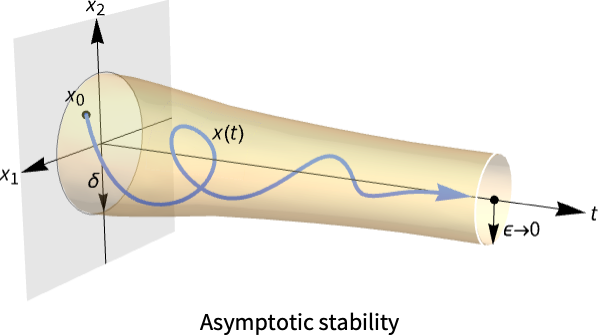
- Stability is also known as asymptotic stability, and fixed points are also known as equilibrium points or stationary points.
- DStabilityConditions is typically used to qualitatively analyze long-term behavior near fixed points. If the system is stable, then solutions converge to the fixed point if you are close enough.
- For a system of differential equations
 , a point
  is a fixed point iff
  . In effect, the initial value
  remains stationary; if you initialize at
  you stay at
  .
. - A fixed point
 is asymptotically stable iff for
  and
and  you have
 ![TemplateBox[{{x, (, t, )}, t, infty}, Limit2Arg]=x^*](Files/DStabilityConditions.en/10.png "TemplateBox[{{x, (, t, )}, t, infty}, Limit2Arg]=x^*") for
for  sufficiently small.
 - DStabilityConditions returns a list of the form {{{
 ,
, ,…},cond},…}, where {
 ,
, ,…} is a fixed point.
 - Systems of higher-order ODEs are treated as systems of first-order ODEs with additional variables corresponding to the higher-order derivatives. In this case. the fixed points are given as nested lists {{x,x',…},{y,y',…},…}.
- DStabilityConditions gives sufficient conditions for local stability of fixed points. For linear systems, these conditions are also conditions for global stability.
- DStabilityConditions works for linear and nonlinear ordinary differential equations.
- The following options can be given:
-
Assumptions $Assumptions assumptions on parameters
Examples
open all close allBasic Examples (5)
Find the fixed point and determine its stability for the equation ![]() :
:
DStabilityConditions[x'[t] == -2x[t], x[t], t]Find the fixed point and determine the stability for the equation ![]() :
:
DStabilityConditions[x'[t] == 2x[t] + 1, x[t], t]Find the fixed points and conditions for stability for the equation ![]() :
:
DStabilityConditions[y'[t] == a y[t], y, t]Plot several solutions for different values of a:
sol = DSolveValue[{y'[t] == a y[t], y[0] == -1}, y[t], t]Table[Plot[sol, {t, 0, 4}, PlotLabel -> Row[{"a=", a}]], {a, {-1.1, 1.1}}]Stability analysis of a two-dimensional system:
DStabilityConditions[{x'[t] == b x[t] + y[t], y'[t] == -2 x[t] + a y[t]}, {x, y}, t]Plot the parameter region for which the system is stable:
RegionPlot[%[[1, 2]], {a, -5, 5}, {b, -5, 5}]Find the fixed points for a nonlinear equation:
points = DFixedPoints[y[t]^2 + 3 y'[t] + y''[t] == 2, y, t]Study the stability of the first point:
DStabilityConditions[y[t]^2 + 3 y'[t] + y''[t] == 2, y, t, {points[[1]]}]Study the stability of the second point:
DStabilityConditions[y[t]^2 + 3 y'[t] + y''[t] == 2, y, t, {points[[2]]}]Scope (25)
Linear Equations (5)
Find the fixed point and determine its stability for the equation ![]() :
:
DStabilityConditions[x'[t] == -3 x[t], x, t]A first-order linear inhomogeneous equation:
DStabilityConditions[y'[t] == a y[t] + 5, y, t]Plot the unstable solution for ![]() :
:
sol = DSolveValue[{y'[t] == a y[t] + 5, y[0] == 1}, y[t], t];
Plot[sol /. a -> 0.5, {t, 0, 10}]
Plot the stable solution for ![]() :
:
sol = DSolveValue[{y'[t] == a y[t] + 5, y[0] == 1}, y[t], t];
Plot[sol /. a -> -0.5, {t, 0, 10}]DStabilityConditions[y''[t] + a y'[t] + b y[t] == 0, y, t]Plot the stability region for parameters ![]() and
and ![]() :
:
RegionPlot[%[[1, 2]], {a, -2, 2}, {b, -2, 2}, Rule[...]]DStabilityConditions[y'''[t] + a y''[t] + b y'[t] + c y[t] == 0, y, t]RegionPlot3D[%[[1, 2]], {b, -2, 2}, {c, -2, 2}, {a, -2, 2}]Higher-order inhomogeneous ODE:
DStabilityConditions[y'''[x] + 5y''[x] + 3y'[x] + 6y[x] == 3, y, x]Solve the ODE using coordinates of the fixed point as initial values:
DSolve[{y'''[x] + 5y''[x] + 3y'[x] + 6y[x] == 3, y[0] == 1 / 2, y'[0] == 0, y''[0] == 0}, y[x], x]Nonlinear Equations (3)
Stability analysis of a nonlinear differential equation:
DStabilityConditions[x'[t] == x[t]^2 + 3x[t], x, t]Use StreamPlot to demonstrate the stability:
StreamPlot[{1, x^2 + 3x}, {t, 0, 10}, {x, -4, 1}]The stability of a first-order nonlinear equation:
DStabilityConditions[x'[t] == x[t]^2 - 5x[t] + 6, x, t]Plot the solution for the initial value ![]() :
:
sol = DSolveValue[{x'[t] == x[t]^2 - 5x[t] + 6, x[0] == 5 / 2}, x[t], t]Plot[sol, {t, 0, 10}, PlotRange -> All]Use StreamPlot to demonstrate the stability at ![]() :
:
StreamPlot[{1, x^2 - 5x + 6}, {t, 0, 10}, {x, 0, 4}]Consider a second-order nonlinear ODE:
eqn = y[x]^2 + 3 y'[x] + y''[x] == 2;DSolve is unable to solve this equation:
DSolve[eqn, y, x]Analyze the stability of the equation using DStabilityConditions:
DStabilityConditions[eqn, y, x]Transform the equation into a system of first-order ODEs:
sys = {y'[x] == y1[x], y[x]^2 + 3 y1[x] + y1'[x] == 2};Plot the trajectories of the system in the ![]() plane:
plane:
StreamPlot[{y1, 2 - y^2 - 3y1}, {y, -3, 3}, {y1, -3, 3}, ...]Linear Systems (12)
A stable linear system of uncoupled equations:
DStabilityConditions[{x'[t] == -x[t], y'[t] == -y[t]}, {x, y}, t]StreamPlot[{-x, -y}, {x, -3, 3}, {y, -3, 3}, ...]An unstable linear system of uncoupled equations:
DStabilityConditions[{x'[t] == x[t], y'[t] == y[t]}, {x, y}, t]StreamPlot[{x, y}, {x, -3, 3}, {y, -3, 3}, ...]The stability of a linear system with constant coefficients:
DStabilityConditions[{x'[t] == -x[t] - y[t], y'[t] == 2x[t] - y[t]}, {x, y}, t]Use StreamPlot to visualize the stability:
StreamPlot[{-x - y, 2x - y}, {x, -3, 3}, {y, -3, 3}, ...]Unstable system with constant coefficients:
DStabilityConditions[{x'[t] == 3x[t] - 4y[t], y'[t] == x[t] - y[t]}, {x, y}, t]StreamPlot[{3x - 4y, x - y}, {x, -3, 3}, {y, -3, 3}, Rule[...]]Stable system with constant coefficients:
DStabilityConditions[{x'[t] == -y[t], y'[t] == x[t]}, {x, y}, t]StreamPlot[{-y, x}, {x, -3, 3}, {y, -3, 3}, Rule[...]]A first-order system with imaginary eigenvalues:
A = {{1, 2}, {-5, -1}};Eigenvalues[A]DStabilityConditions[Thread[{x'[t], y'[t]} == A.{x[t], y[t]}], {x, y}, t]Use StreamPlot to visualize the stability:
StreamPlot[A.{x, y}, {x, -3, 3}, {y, -3, 3}, Rule[...]]Inhomogeneous unstable system:
DStabilityConditions[{x'[t] == x[t] + y[t] - 2, y'[t] == x[t] - y[t]}, {x, y}, t]StreamPlot[{x + y - 2, x - y}, {x, -3, 3}, {y, -3, 3}, Rule[...]]DStabilityConditions[{x'[t] == -x[t] - y[t] - 1, y'[t] == 2x[t] - y[t] + 5}, {x, y}, t]StreamPlot[{-x - y - 1, 2x - y + 5}, {x, -3, 3}, {y, -3, 3}, Rule[...]]sol = DSolveValue[{x'[t] == -x[t] - y[t] - 1, y'[t] == 2x[t] - y[t] + 5, x[0] == 2, y[0] == 0}, {x[t], y[t]}, t]Plot[sol, {t, 0, 10}]For the system of two second-order ODEs, the fixed point is a nested list {{y,y'},{z,z'}}:
DStabilityConditions[{-z[t] - 3 y'[t] + y''[t] == 2, z''[t] == y[t] + z'[t] - z[t] - 3}, {y, z}, t]Linear system with symbolic coefficients:
DStabilityConditions[{x'[t] == β y[t] + α, y'[t] == δ x[t] - γ}, {x, y}, t]Use Assumptions to simplify the stability conditions:
DStabilityConditions[{x'[t] == β y[t] + α, y'[t] == δ x[t] - γ}, {x, y}, t, Assumptions -> β > 0 && δ > 0]DStabilityConditions[{Derivative[1][x][t] == 2 x[t] - 5 y[t], Derivative[1][y][t] == x[t] - 2 y[t], Derivative[1][u][t] == u[t] + 2 v[t], Derivative[1][v][t] == -5 u[t] - v[t]}, {x, y, u, v}, t]sol = DSolveValue[{Derivative[1][x][t] == 2 x[t] - 5 y[t], Derivative[1][y][t] == x[t] - 2 y[t], Derivative[1][u][t] == u[t] + 2 v[t], Derivative[1][v][t] == -5 u[t] - v[t]}, {x[t], y[t], u[t], v[t]}, t]Plot[Evaluate[sol /. {C[1] -> 1, C[2] -> 2, C[3] -> 3, C[4] -> 4}], {t, 0, 10}]Analyze the stability of a 10×10 linear system with random constant coefficients:
SeedRandom[1234];
m = RandomInteger[10, {10, 10}];
g = RandomInteger[10, 10];dep = {x1[t], x2[t], x3[t], x4[t], x5[t], x6[t], x7[t], x8[t], x9[t], x10[t]};sys = Thread[D[dep, t] == m.dep + g];DStabilityConditions[sys, dep, t]Nonlinear Systems (5)
A nonlinear first-order system:
DStabilityConditions[{x'[t] == −x[t] + 2x[t] y[t], y'[t] == y[t]−x[t]^2−y[t]^2}, {x, y}, t]Use StreamPlot to visualize the stability:
StreamPlot[{−x + 2x y, y−x^2−y^2}, {x, -2, 2}, {y, -1, 2}, Rule[...]]A nonlinear system with periodic fixed points:
DStabilityConditions[{x'[t] == y[t], y'[t] == Sin[x[t]]}, {x, y}, t]StreamPlot[{y, Sin[x]}, {x, -4Pi, 4Pi}, {y, -6, 6}, Rule[...]]A nonlinear system with unstable fixed point at origin:
DStabilityConditions[{y[t] + x[t](1−x[t]^2−y[t]^2) == x'[t], −x[t] + y[t](1−x[t]^2−y[t]^2) == y'[t]}, {x, y}, t]StreamPlot[{y + x(1−x^2−y^2), −x + y(1−x^2−y^2)}, {x, -3, 3}, {y, -3, 3}, Rule[...]]Higher-order nonlinear system:
DStabilityConditions[{x''[t] == -2(x[t]^2 + y[t]^2)x'[t] - x[t] - 1, y''[t] == -2(x[t]^2 + y[t]^2)y'[t] - y[t]}, {x, y}, t]A nonlinear system of three ODEs:
DStabilityConditions[{σ(−x[t] + y[t]) == x'[t], r x[t]−y[t]−x[t] z[t] == y'[t], −b z[t] + x[t] y[t] == z'[t]}, {x, y, z}, t]Simplify[%, b > 0 && r > 1 && σ > 0]Options (2)
Assumptions (2)
Without Assumptions, there are conditions on parameters for stability:
DStabilityConditions[y'[t] == a y[t], y, t]Using Assumptions can often result in simplified conditions:
DStabilityConditions[y'[t] == a y[t], y, t, Assumptions -> a < 0]A system of two nonlinear equations has an infinite number of periodic fixed points:
DStabilityConditions[{x'[t] == y[t], y'[t] == Sin[x[t]]}, {x, y}, t]Use Assumptions to specify the range of a dependent variable:
DStabilityConditions[{x'[t] == y[t], y'[t] == Sin[x[t]]}, {x, y}, t, Assumptions -> -4 < x[t] < 4]Applications (11)
Physics (5)
Do stability analysis for the spring-mass system with damping:
DStabilityConditions[m u''[t] + c u'[t] + k u[t] == 0, u, t]Use assumptions to simplify the stability conditions:
DStabilityConditions[m u''[t] + c u'[t] + k u[t] == 0, u, t, Assumptions -> m > 0 && c > 0 && k > 0]Solve the spring-mass system equation:
sol = DSolveValue[{m u''[t] + c u'[t] + k u[t] == 0, u[0] == 1, u'[0] == 0}, u[t], t]Plot the solution for given values of parameters:
Plot[sol /. {m -> 1, k -> 1, c -> 0.5}, {t, 0, 20}, PlotRange -> All]Do stability analysis for the electric circuit equation:
DStabilityConditions[l i''[t] + r i'[t] + (1/c) i[t] == 0, i, t]Solve the electric circuit equation:
sol = DSolveValue[{l i''[t] + r i'[t] + (1/c) i[t] == 0, i[0] == 1, i'[0] == 0}, i[t], t]Plot the solution for given values of parameters:
Plot[sol /. {r -> 0.1, l -> 5 10^-2, c -> 0.1}, {t, 0, 10}, PlotRange -> All]Stability analysis for the damped pendulum equation:
DStabilityConditions[θ''[t] + 1 / 5 θ'[t] + 9 Sin[θ[t]] == 0, θ, t]Plot the phase portrait of the system:
StreamPlot[{θ1, -1 / 5θ1 - 9Sin[θ]}, {θ, -3Pi, 3Pi}, {θ1, -10, 10}, ...]Plot the solution for the initial conditions ![]() ,
, ![]() :
:
sol = NDSolve[{θ''[t] + 1 / 5 θ'[t] + 9 Sin[θ[t]] == 0, θ[0] == Pi / 2, θ'[0] == 0}, θ[t], {t, 0, 20}];
Plot[θ[t] /. sol, {t, 0, 20}, PlotRange -> All]
Stable system of Lorenz equations:
σ = 10;
b = 8 / 3;
r = 15;
eqns = {σ(−x[t] + y[t]) == x'[t], r x[t]−y[t]−x[t] z[t] == y'[t], −b z[t] + x[t] y[t] == z'[t]};DStabilityConditions[eqns, {x, y, z}, t]Use StreamPlot3D to visualize the Lorenz attractors:
StreamPlot3D[{σ(−x + y), r x−y−x z, −b z + x y}, {x, -10, 10}, {y, -10, 10}, {z, 0, 20}]Unstable system of Lorenz equations:
σ = 10;
b = 8 / 3;
r = 28;
eqns = {σ(−x[t] + y[t]) == x'[t], r x[t]−y[t]−x[t] z[t] == y'[t], −b z[t] + x[t] y[t] == z'[t]};DStabilityConditions[eqns, {x, y, z}, t]Solve the system and plot the solution:
sol = NDSolve[{eqns, x[0] == 10, y[0] == 10, z[0] == 20}, {x[t], y[t], z[t]}, {t, 0, 200}];ParametricPlot3D[{x[t], y[t], z[t]} /. sol, {t, 0, 200}, ...]Biology and Ecology (3)
Stability analysis for the predator-prey model (Lotka–Volterra equation):
DStabilityConditions[{x'[t] == x[t](1 - 1 / 2y[t]), y'[t] == y[t](-3 / 4 + 1 / 4x[t])}, {x, y}, t]Plot the phase portrait of the system:
StreamPlot[{x(1 - 1 / 2y), y(-3 / 4 + 1 / 4x)}, {x, 0, 8}, {y, 0, 4}, Rule[...]]Solve the system for the initial conditions ![]() ,
, ![]() :
:
sol = NDSolve[{x'[t] == x[t](1 - 1 / 2y[t]), y'[t] == y[t](-3 / 4 + 1 / 4x[t]), x[0] == 2, y[0] == 1}, {x[t], y[t]}, {t, 0, 30}]Plot[Evaluate[{x[t], y[t]} /. sol], {t, 0, 30}, ...]The Rosenzweig–MacArthur predator-prey model:
eqns = {n'[t] == n[t](1 - n[t] / k) - an p[t]n[t] / (n[t] + h), p'[t] == p[t](ap n[t] / (n[t] + h) - m)};params = {an -> 1, ap -> 2, h -> 1, m -> 1, k -> 4};DStabilityConditions[eqns /. params, {n, p}, t]StreamPlot[{n(1 - n / k) - an p n / (n + h), p(ap n / (n + h) - m)} /. params, {n, 0, 4}, {p, 0, 4}, Rule[...]]The chemostat model represents biological systems in which microorganisms grow on abiotic resources:
model = {x'[t] == (k x[t]y[t]/1 + y[t]) - x[t], y'[t] == -(x[t]y[t]/1 + y[t]) - y[t] + q};Analyze the stability of the model for ![]() and
and ![]() :
:
DStabilityConditions[model /. {k -> 2, q -> 2}, {x, y}, t]StreamPlot[{(k x y/1 + y) - x, -(x y/1 + y) - y + q} /. {k -> 2, q -> 2}, {x, 0, 4}, {y, 0, 3}, Rule[...]]Chemistry (1)
The Brusselator is a theoretical model for a type of autocatalytic reaction.
The rate equations of the Brusselator model:
sys = {x'[t] == x[t]^2y[t] - (b + 1)x[t] + a, y'[t] == -x[t]^2y[t] + b x[t]};Find the fixed point of the system:
DFixedPoints[sys, {x, y}, t]The point is stable if b<1+a2:
DStabilityConditions[sys /. {a -> 1, b -> 3 / 2}, {x, y}, t]StreamPlot[{x^2y - (b + 1)x + a, -x^2y + b x} /. {a -> 1, b -> 3 / 2}, {x, 0, 3}, {y, 0, 4}, Rule[...]]The point is unstable if b>1+a2:
DStabilityConditions[sys /. {a -> 1, b -> 5 / 2}, {x, y}, t]StreamPlot[{x^2y - (b + 1)x + a, -x^2y + b x} /. {a -> 1, b -> 5 / 2}, {x, 0, 3}, {y, 0, 4}, Rule[...]]Control Systems (2)
Analyze a satellite's attitude dynamics starting from Euler's equations of motion:
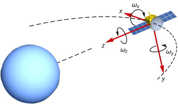
Euler’s equations with principal moments of inertia ![]() ,
, ![]() ,
, ![]() :
:
eqns = Table[Subscript[j, i[[1]]] Subscript[ω, i[[1]]]'[t] - (Subscript[j, i[[2]]] - Subscript[j, i[[3]]])Subscript[ω, i[[2]]][t]Subscript[ω, i[[3]]][t] == Subscript[τ, i[[1]]][t], {i, {{x, y, z}, {y, z, x}, {z, x, y}}}] /. {Subscript[j, x] -> 300, Subscript[j, y] -> 320, Subscript[j, z] -> 270}Analyze the stability of the equation for fixed values of ![]() ,
, ![]() ,
, ![]() :
:
DStabilityConditions[eqns /. {Subscript[τ, x][t] -> -27 / 400, Subscript[τ, y][t] -> 3 / 200, Subscript[τ, z][t] -> 1 / 50}, {Subscript[ω, x], Subscript[ω, y], Subscript[ω, z]}, t]Choose the fixed point as an operating point:
opPt = {Subscript[ω, x0] -> (1/30Sqrt[3]), Subscript[ω, y0] -> (3Sqrt[3]/100), Subscript[ω, z0] -> (3Sqrt[3]/200), Subscript[τ, x0] -> -(27/400), Subscript[τ, y0] -> (3/200), Subscript[τ, z0] -> (1/50)};Construct a state-space model:
ssm = StateSpaceModel[eqns, {{Subscript[ω, x][t], Subscript[ω, x0]}, {Subscript[ω, y][t], Subscript[ω, y0]}, {Subscript[ω, z][t], Subscript[ω, z0]}}, {{Subscript[τ, x][t], Subscript[τ, x0]}, {Subscript[τ, y][t], Subscript[τ, y0]}, {Subscript[τ, z][t], Subscript[τ, z0]}}, {Subscript[ω, x][t], Subscript[ω, y][t], Subscript[ω, z][t]}, t, SystemsModelLabels -> {{Subscript[τ, x], Subscript[τ, y], Subscript[τ, z]}, {Subscript[ω, x], Subscript[ω, y], Subscript[ω, z]}, {Subscript[ω, x], Subscript[ω, y], Subscript[ω, z]}}] /. opPtThe satellite’s attitude is unregulated if disturbed:
OutputResponse[{ssm, {0.2, -0.1, 0.35}}, {0, 0, 0}, {t, 0, 3000}];
Plot[%, {t, 0, 3000}, PlotRange -> All, PlotLegends -> {Subscript[ω, x], Subscript[ω, y], Subscript[ω, z]}]
Verify the controllability of the model:
ControllableModelQ[ssm]Study an inverted pendulum using the Lagrangian:
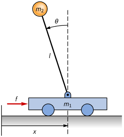
Subscript[r, p] = Composition[TranslationTransform[{x[t], 0, 0}], RotationTransform[θ[t], {0, 0, 1}]][{0, 1, 0}]Subscript[v, p] = D[Subscript[r, p], t]The kinetic energy of the cart and pendulum:
𝒦 = (1/2)Subscript[m, 1] x'[t]^2 + (1/2)Subscript[m, 2]Subscript[v, p].Subscript[v, p]The potential energy of the pendulum:
𝒰 = Subscript[m, 2]g Subscript[r, p][[2]]ℒ = 𝒦 - 𝒰{Subscript[f, x], Subscript[f, θ]} = D[f[t] δx - Subscript[b, x]x'[t]δx - Subscript[b, θ]θ'[t]δθ, {{δx, δθ}}]eqns = Table[Subscript[∂, t]D[ℒ, q'[t]] - D[ℒ, q[t]] == Subscript[f, q], {q, {x, θ}}]//Simplifyssm = StateSpaceModel[eqns, {x[t], x'[t], θ[t], θ'[t]}, f[t], {x[t], θ[t]}, t, SystemsModelLabels -> {f, {x, θ}, {x, Derivative[1][x], θ, Derivative[1][θ]}}]The non-positive eigenvalues make it an unstable system:
Eigenvalues[First[Normal[ssm /. {Subscript[m, 1] -> 1 / 2, Subscript[m, 2] -> 1 / 10, l -> 3 / 10, g -> 10, Subscript[b, x] -> 15 / 100, Subscript[b, θ] -> 1 / 100}]]]//NDFixedPoints[eqns /. {Subscript[m, 1] -> 1 / 2, Subscript[m, 2] -> 1 / 10, l -> 3 / 10, g -> 10, Subscript[b, x] -> 15 / 100, Subscript[b, θ] -> 1 / 100, f[t] -> 0}, {x, θ}, t]DStabilityConditions[eqns /. {Subscript[m, 1] -> 1 / 2, Subscript[m, 2] -> 1 / 10, l -> 3 / 10, g -> 10, Subscript[b, x] -> 15 / 100, Subscript[b, θ] -> 1 / 100, f[t] -> 0}, {x, θ}, t, {{1, 0, 2Pi, 0}, {1, 0, 3Pi, 0}}]Properties & Relations (9)
DStabilityConditions returns fixed points and stability conditions for differential equations:
DStabilityConditions[y'[t] == a y[t], y, t]DStabilityConditions[y'[t] == (1/2)y[t], y, t]DStabilityConditions[y'[t] == -(1/2) y[t], y, t]Use DFixedPoints to find all fixed points of a differential equation:
DFixedPoints[y'[t] == 2 y[t](1 - y[t]), y[t], t]Analyze the stability at specific fixed points:
DStabilityConditions[y'[t] == 2 y[t](1 - y[t]), y[t], t, {{0}}]DStabilityConditions[y'[t] == 2 y[t](1 - y[t]), y[t], t, {{1}}]Use DFixedPoints to find all fixed points of a nonlinear ODE:
points = DFixedPoints[x'[t] == x[t]^2 + 3x[t], x, t]Use Solve to find the fixed points:
Solve[x^2 + 3x == 0, x]Linearize the equation near the first fixed point:
f1 = D[x^2 + 3x, x] /. x -> points[[1, 1]];
leqn1 = x'[t] == f1 x[t]
Check the stability near the first fixed point:
DStabilityConditions[leqn1, x, t][[1, 2]]Linearize the equation near the second fixed point:
f1 = D[x^2 + 3x, x] /. x -> points[[2, 1]];
leqn2 = x'[t] == f1 x[t]
Check the stability near the second fixed point:
DStabilityConditions[leqn2, x, t][[1, 2]]Determine the stability of a nonlinear equation using DStabilityConditions:
DStabilityConditions[x'[t] == x[t]^2 + 3x[t], x, t]The fixed points for the n![]() -order differential equation are n-dimensional vectors:
-order differential equation are n-dimensional vectors:
DStabilityConditions[y''[t] + y'[t] + 3 y[t] == 5, y, t]The fixed points for the system of n first-order differential equations are n-dimensional vectors:
DStabilityConditions[{y'[t] + z[t] == 3, y[t] + 2 z'[t] == 1}, {y[t], z[t]}, t]Analyze the stability of a system of two ODEs:
DStabilityConditions[{x'[t] == -x[t] - y[t] - 1, y'[t] == 2x[t] - y[t] + 5}, {x, y}, t]Use DSolveValue to solve the system using a fixed point as initial condition:
sol = DSolveValue[{x'[t] == -x[t] - y[t] - 1, y'[t] == 2x[t] - y[t] + 5, x[0] == -2, y[0] == 1}, {x[t], y[t]}, t]//SimplifyUse DSolveValue to solve the system for given initial conditions:
sol = DSolveValue[{x'[t] == -x[t] - y[t] - 1, y'[t] == 2x[t] - y[t] + 5, x[0] == 3, y[0] == -2}, {x[t], y[t]}, t]//SimplifyPlot[Evaluate[sol], {t, 0, 20}]Analyze the stability of a nonlinear ODE:
DStabilityConditions[x'[t] == (1/2)x[t](1 - x[t]), x, t]Solve the ODE using NDSolve:
sol = NDSolve[{x'[t] == (1/2)x[t](1 - x[t]), x[0] == 0.5}, x[t], {t, 0, 20}]Plot[x[t] /. sol, {t, 0, 20}, PlotRange -> All]Analyze the stability of a nonlinear ODE:
DStabilityConditions[2 y'[x] - y[x] ^ 2 == -1, y, x]Calculate an asymptotic solution of the ODE using the first fixed point as initial condition:
AsymptoticDSolveValue[{2 y'[x] - y[x] ^ 2 == -1, y[0] == -1}, y, {x, 0, 6}]Calculate an asymptotic solution of the ODE for another initial condition:
AsymptoticDSolveValue[{2 y'[t] - y[t] ^ 2 == -1, y[0] == -1 + ϵ}, y, t, {ϵ, 0, 2}]Limit[%, t -> Infinity]AsymptoticDSolveValue[{2 y'[t] - y[t] ^ 2 == -1, y[0] == 1 + ϵ}, y, t, {ϵ, 0, 2}]Limit[%, t -> Infinity, Assumptions -> Im[ϵ] == 0]Find the fixed points for the system of two nonlinear ODEs:
points = DFixedPoints[{x'[t] == x[t](2−x[t]−y[t]), y'[t] == −x[t] + 3y[t]−2x[t] y[t]}, {x, y}, t]Calculate the Jacobian matrix of the system:
(jacobian = D[{x(2−x−y), −x + 3y−2x y}, {{x, y}}])//MatrixFormCalculate the eigenvalues of the Jacobian matrix for each fixed point:
eig1 = Eigenvalues[jacobian /. Thread[{x, y} -> points[[1]]]]eig2 = Eigenvalues[jacobian /. Thread[{x, y} -> points[[2]]]]eig3 = Eigenvalues[jacobian /. Thread[{x, y} -> points[[3]]]]The system is locally stable near the fixed point if all of the eigenvalues have negative real parts:
Re[#] < 0& /@ eig1Re[#] < 0& /@ eig2Re[#] < 0& /@ eig3Check the stability of the points using DStabilityConditions:
DStabilityConditions[{x'[t] == x[t](2−x[t]−y[t]), y'[t] == −x[t] + 3y[t]−2x[t] y[t]}, {x, y}, t]Possible Issues (2)
Sometimes the conditions for stability are not the simplest possible:
res = DStabilityConditions[{σ(−x[t] + y[t]) == x'[t], r x[t]−y[t]−x[t] z[t] == y'[t], −b z[t] + x[t] y[t] == z'[t]}, {x, y, z}, t]Additional simplification can be achieved by further processing:
Simplify[#, b > 0 && r > 1 && σ > 0]& /@ resDStabilityConditions fails because the given point is not a fixed point:
DStabilityConditions[y'[t] == y[t](1 - y[t]), y, t, {{2}}]Use DFixedPoints to find all fixed points of the equation first:
points = DFixedPoints[y'[t] == 3 y[t](1 - y[t]), y, t]DStabilityConditions[y'[t] == 3 y[t](1 - y[t]), y, t, {points[[1]]}]DStabilityConditions[y'[t] == 3 y[t](1 - y[t]), y, t, {points[[2]]}]Neat Examples (2)
The van der Pol oscillator is a non-conservative, oscillating system with nonlinear damping:
sys = {x'[t] == y[t], y'[t] == -x[t] + μ (1 - x[t]^2)y[t]};Analyze the stability of the system:
DStabilityConditions[sys, {x, y}, t]Animate the trajectories of the system for various values of the parameter ![]() :
:
Animate[StreamPlot[{y, -x + μ (1 - x^2)y}, {x, -4, 4}, {y, -4, 4}], {μ, 0.01, 4}]The FitzHugh–Nagumo model is an example of a relaxation oscillator:
sys = {x'[t] == 3y[t] - x[t](x[t]^2 - 3) + s, y'[t] == (7 - 10x[t] - 8y[t]) / 30};If the external stimulus s exceeds a certain threshold value, the system will exhibit a characteristic excursion in phase space, before the variables x and y relax back to their rest values.
DStabilityConditions[sys /. s -> 1 / 100, {x, y}, t]Visualize the trajectories of the system for various values of the parameter s:
Animate[StreamPlot[{3y - x(x^2 - 3) + s, (7 - 10x - 8y) / 30}, {x, -3, 3}, {y, -3, 3}], {s, 0.01, 4}]Text
Wolfram Research (2024), DStabilityConditions, Wolfram Language function, https://reference.wolfram.com/language/ref/DStabilityConditions.html.
CMS
Wolfram Language. 2024. "DStabilityConditions." Wolfram Language & System Documentation Center. Wolfram Research. https://reference.wolfram.com/language/ref/DStabilityConditions.html.
APA
Wolfram Language. (2024). DStabilityConditions. Wolfram Language & System Documentation Center. Retrieved from https://reference.wolfram.com/language/ref/DStabilityConditions.html