Wolfram言語＆システムドキュメントセンター

DStabilityConditions

DStabilityConditions[eqn,x[t],t]

微分方程式の不動点と安定条件を与える．

DStabilityConditions[{eqn₁,eqn₂,…},{x₁[t],x₂[t],…},t]

微分方程式系の不動点と安定条件を与える．

DStabilityConditions[{eqn₁,eqn₂,…},{x₁[t],x₂[t],…},t,{pnt₁,pnt₂,…}]

指定された不動点についてのみ安定条件を与える．

詳細とオプション

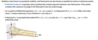
安定性は近似安定性として，不動点は平衡点または停留点としても知られている．
DStabilityConditionsは，不動点近くの長期的な挙動の定性的解析によく使われる．系が安定しているなら，十分近ければ解は不動点に収束する．
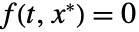
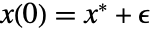
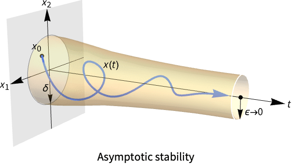
微分方程式の系の点は，のときかつそのときに限って不動点である．事実，初期値は不動点のままで，で初期化したならに留まる．
不動点は，でのときに限り，漸近的に安定している．十分小さいについて $TemplateBox[{{x, (, t, )}, t, infty}, Limit2Arg]=x^*$ である．

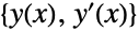
DStabilityConditionsは{{{,,…},cond},…} の形のリストを返す．ただし，{,,…}は不動点である．
高階常微分方程式系は，高階微分に対応する変数を追加した一次常微分方程式系として扱われる．この場合，不動点はネストしたリスト{{x,x',…},{y,y',…},…}として与えられる．
DStabilityConditionsは不動点の局所的な安定性に十分な条件を与える．線形系については，これらの条件は大域的安定性の条件でもある．
DStabilityConditionsは線形および非線形の常微分方程式に使うことができる．
次は，使用できるオプションである．
Assumptions $Assumptions パラメータについての仮定

例題

すべて開くすべて閉じる

例 (5)

方程式の不動点を求め，その安定性を判定する：

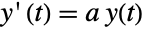
Wolfram Language code: DStabilityConditions[x'[t] == -2x[t], x[t], t]

方程式の不動点を求め，その安定性を判定する：

Wolfram Language code: DStabilityConditions[x'[t] == 2x[t] + 1, x[t], t]

方程式の不動点と安定性の条件を求める：

Wolfram Language code: DStabilityConditions[y'[t] == a y[t], y, t]

a のさまざまな値についていくつかの解をプロットする：

Wolfram Language code: sol = DSolveValue[{y'[t] == a y[t], y[0] == -1}, y[t], t]

Wolfram Language code: Table[Plot[sol, {t, 0, 4}, PlotLabel -> Row[{"a=", a}]], {a, {-1.1, 1.1}}]

二次元の系についての安定性解析：

Wolfram Language code: DStabilityConditions[{x'[t] == b x[t] + y[t], y'[t] == -2 x[t] + a y[t]}, {x, y}, t]

系が安定するパラメータ領域をプロットする：

Wolfram Language code: RegionPlot[%[[1, 2]], {a, -5, 5}, {b, -5, 5}]

非線形方程式の不動点を求める：

Wolfram Language code: points = DFixedPoints[y[t]^2 + 3 y'[t] + y''[t] == 2, y, t]

最初の点の安定性を調べる：

Wolfram Language code: DStabilityConditions[y[t]^2 + 3 y'[t] + y''[t] == 2, y, t, {points[[1]]}]

2番目の点の安定性を調べる：

Wolfram Language code: DStabilityConditions[y[t]^2 + 3 y'[t] + y''[t] == 2, y, t, {points[[2]]}]

スコープ (25)

線形方程式 (5)

方程式の不動点を求め，その安定性を判定する：

Wolfram Language code: DStabilityConditions[x'[t] == -3 x[t], x, t]

一次線形非同次方程式：

Wolfram Language code: DStabilityConditions[y'[t] == a y[t] + 5, y, t]

のときの不安定解をプロットする：

Wolfram Language code:

sol = DSolveValue[{y'[t] == a y[t] + 5, y[0] == 1}, y[t], t];
Plot[sol /. a -> 0.5, {t, 0, 10}]

のときの安定解をプロットする：

Wolfram Language code:

sol = DSolveValue[{y'[t] == a y[t] + 5, y[0] == 1}, y[t], t];
Plot[sol /. a -> -0.5, {t, 0, 10}]

二次線形方程式：

Wolfram Language code: DStabilityConditions[y''[t] + a y'[t] + b y[t] == 0, y, t]

パラメータとについて，安定領域をプロットする：

Wolfram Language code: RegionPlot[%[[1, 2]], {a, -2, 2}, {b, -2, 2}, Rule[...]]

三次線形方程式：

Wolfram Language code: DStabilityConditions[y'''[t] + a y''[t] + b y'[t] + c y[t] == 0, y, t]

安定領域をプロットする：

Wolfram Language code: RegionPlot3D[%[[1, 2]], {b, -2, 2}, {c, -2, 2}, {a, -2, 2}]

より高次の非同次常微分方程式：

Wolfram Language code: DStabilityConditions[y'''[x] + 5y''[x] + 3y'[x] + 6y[x] == 3, y, x]

不動点の座標を初期値として使って常微分方程式を解く：

Wolfram Language code: DSolve[{y'''[x] + 5y''[x] + 3y'[x] + 6y[x] == 3, y[0] == 1 / 2, y'[0] == 0, y''[0] == 0}, y[x], x]

非線形方程式 (3)

非線形微分方程式の安定性解析：

Wolfram Language code: DStabilityConditions[x'[t] == x[t]^2 + 3x[t], x, t]

StreamPlotを使って安定性を示す：

Wolfram Language code: StreamPlot[{1, x^2 + 3x}, {t, 0, 10}, {x, -4, 1}]

一次非線形方程式の安定性：

Wolfram Language code: DStabilityConditions[x'[t] == x[t]^2 - 5x[t] + 6, x, t]

初期値についての解をプロットする：

Wolfram Language code: sol = DSolveValue[{x'[t] == x[t]^2 - 5x[t] + 6, x[0] == 5 / 2}, x[t], t]

Wolfram Language code: Plot[sol, {t, 0, 10}, PlotRange -> All]

StreamPlotを使ってにおける安定性を示す：

Wolfram Language code: StreamPlot[{1, x^2 - 5x + 6}, {t, 0, 10}, {x, 0, 4}]

二次非線形常微分方程式について考える：

Wolfram Language code: eqn = y[x]^2 + 3 y'[x] + y''[x] == 2;

DSolveは，この方程式を解くことができない：

Wolfram Language code: DSolve[eqn, y, x]

DStabilityConditionsを使ってこの方程式の安定性を解析する：

Wolfram Language code: DStabilityConditions[eqn, y, x]

この方程式を一次常微分方程式の系に変換する：

Wolfram Language code: sys = {y'[x] == y1[x], y[x]^2 + 3 y1[x] + y1'[x] == 2};

平面におけるこの系の軌跡をプロットする：

Wolfram Language code: StreamPlot[{y1, 2 - y^2 - 3y1}, {y, -3, 3}, {y1, -3, 3}, ...]

線形系 (12)

非連立方程式の安定した線形系：

Wolfram Language code: DStabilityConditions[{x'[t] == -x[t], y'[t] == -y[t]}, {x, y}, t]

系の軌跡：

Wolfram Language code: StreamPlot[{-x, -y}, {x, -3, 3}, {y, -3, 3}, ...]

非連立方程式の不安定な線形系：

Wolfram Language code: DStabilityConditions[{x'[t] == x[t], y'[t] == y[t]}, {x, y}, t]

系の軌跡：

Wolfram Language code: StreamPlot[{x, y}, {x, -3, 3}, {y, -3, 3}, ...]

定数係数を持つ線形系の安定性：

Wolfram Language code: DStabilityConditions[{x'[t] == -x[t] - y[t], y'[t] == 2x[t] - y[t]}, {x, y}, t]

StreamPlotを使って安定性を可視化する：

Wolfram Language code: StreamPlot[{-x - y, 2x - y}, {x, -3, 3}, {y, -3, 3}, ...]

定数係数を持つ不安定な系：

Wolfram Language code: DStabilityConditions[{x'[t] == 3x[t] - 4y[t], y'[t] == x[t] - y[t]}, {x, y}, t]

Wolfram Language code: StreamPlot[{3x - 4y, x - y}, {x, -3, 3}, {y, -3, 3}, Rule[...]]

定数係数を持つ安定した系：

Wolfram Language code: DStabilityConditions[{x'[t] == -y[t], y'[t] == x[t]}, {x, y}, t]

Wolfram Language code: StreamPlot[{-y, x}, {x, -3, 3}, {y, -3, 3}, Rule[...]]

虚数の固有値を持つ一次の系：

Wolfram Language code: A = {{1, 2}, {-5, -1}};

Wolfram Language code: Eigenvalues[A]

Wolfram Language code: DStabilityConditions[Thread[{x'[t], y'[t]} == A.{x[t], y[t]}], {x, y}, t]

StreamPlotを使って安定性を可視化する：

Wolfram Language code: StreamPlot[A.{x, y}, {x, -3, 3}, {y, -3, 3}, Rule[...]]

非同次の不安定な系：

Wolfram Language code: DStabilityConditions[{x'[t] == x[t] + y[t] - 2, y'[t] == x[t] - y[t]}, {x, y}, t]

Wolfram Language code: StreamPlot[{x + y - 2, x - y}, {x, -3, 3}, {y, -3, 3}, Rule[...]]

非同次の安定した系：

Wolfram Language code: DStabilityConditions[{x'[t] == -x[t] - y[t] - 1, y'[t] == 2x[t] - y[t] + 5}, {x, y}, t]

Wolfram Language code: StreamPlot[{-x - y - 1, 2x - y + 5}, {x, -3, 3}, {y, -3, 3}, Rule[...]]

解をプロットする：

Wolfram Language code: sol = DSolveValue[{x'[t] == -x[t] - y[t] - 1, y'[t] == 2x[t] - y[t] + 5, x[0] == 2, y[0] == 0}, {x[t], y[t]}, t]

Wolfram Language code: Plot[sol, {t, 0, 10}]

2つの2階常微分方程式の系について，不動点はネストしたリスト{{y,y'},{z,z'}}で与えられる：

Wolfram Language code: DStabilityConditions[{-z[t] - 3 y'[t] + y''[t] == 2, z''[t] == y[t] + z'[t] - z[t] - 3}, {y, z}, t]

記号係数を持つ線形系：

Wolfram Language code: DStabilityConditions[{x'[t] == β y[t] + α, y'[t] == δ x[t] - γ}, {x, y}, t]

Assumptionsを使って安定性条件を簡約する：

Wolfram Language code: DStabilityConditions[{x'[t] == β y[t] + α, y'[t] == δ x[t] - γ}, {x, y}, t, Assumptions -> β > 0 && δ > 0]

4つの線形常微分方程式の系：

Wolfram Language code:

DStabilityConditions[{Derivative[1][x][t] == 2 x[t] - 5 y[t], Derivative[1][y][t] == x[t] - 2 y[t], Derivative[1][u][t] == u[t] + 2 v[t], Derivative[1][v][t] == -5 u[t] - v[t]}, {x, y, u, v}, t]

解をプロットする：

Wolfram Language code:

sol = DSolveValue[{Derivative[1][x][t] == 2 x[t] - 5 y[t], Derivative[1][y][t] == x[t] - 2 y[t], Derivative[1][u][t] == u[t] + 2 v[t], Derivative[1][v][t] == -5 u[t] - v[t]}, {x[t], y[t], u[t], v[t]}, t]

Wolfram Language code: Plot[Evaluate[sol /. {C[1] -> 1, C[2] -> 2, C[3] -> 3, C[4] -> 4}], {t, 0, 10}]

ランダムな定数係数を持つ10×10線形系の安定性を解析する：

Wolfram Language code:

SeedRandom[1234];
m = RandomInteger[10, {10, 10}];
g = RandomInteger[10, 10];

Wolfram Language code: dep = {x1[t], x2[t], x3[t], x4[t], x5[t], x6[t], x7[t], x8[t], x9[t], x10[t]};

Wolfram Language code: sys = Thread[D[dep, t] == m.dep + g];

Wolfram Language code: DStabilityConditions[sys, dep, t]

非線形系 (5)

非線形の一次の系：

Wolfram Language code: DStabilityConditions[{x'[t] == −x[t] + 2x[t] y[t], y'[t] == y[t]−x[t]^2−y[t]^2}, {x, y}, t]

StreamPlotを使って安定性を可視化する：

Wolfram Language code: StreamPlot[{−x + 2x y, y−x^2−y^2}, {x, -2, 2}, {y, -1, 2}, Rule[...]]

周期的な不動点を持つ非線形系：

Wolfram Language code: DStabilityConditions[{x'[t] == y[t], y'[t] == Sin[x[t]]}, {x, y}, t]

Wolfram Language code: StreamPlot[{y, Sin[x]}, {x, -4Pi, 4Pi}, {y, -6, 6}, Rule[...]]

原点に不安定な不動点を持つ非線形系：

Wolfram Language code:

DStabilityConditions[{y[t] + x[t](1−x[t]^2−y[t]^2) == x'[t], −x[t] + y[t](1−x[t]^2−y[t]^2) == y'[t]}, {x, y}, t]

Wolfram Language code: StreamPlot[{y + x(1−x^2−y^2), −x + y(1−x^2−y^2)}, {x, -3, 3}, {y, -3, 3}, Rule[...]]

高階非線形系：

Wolfram Language code:

DStabilityConditions[{x''[t] == -2(x[t]^2 + y[t]^2)x'[t] - x[t] - 1, y''[t] == -2(x[t]^2 + y[t]^2)y'[t] - y[t]}, {x, y}, t]

3つの常微分方程式の非線形系：

Wolfram Language code:

DStabilityConditions[{σ(−x[t] + y[t]) == x'[t], r x[t]−y[t]−x[t] z[t] == y'[t], −b z[t] + x[t] y[t] == z'[t]}, {x, y, z}, t]

結果を簡約する：

Wolfram Language code: Simplify[%, b > 0 && r > 1 && σ > 0]

オプション (2)

Assumptions (2)

Assumptionsがないと，安定性についてのパラメータの条件が付く：

Wolfram Language code: DStabilityConditions[y'[t] == a y[t], y, t]

Assumptionsを使うと，条件が簡約されることが多い：

Wolfram Language code: DStabilityConditions[y'[t] == a y[t], y, t, Assumptions -> a < 0]

2つの非線形方程式の系は無数の周期的不動点を持つ：

Wolfram Language code: DStabilityConditions[{x'[t] == y[t], y'[t] == Sin[x[t]]}, {x, y}, t]

Assumptionsを使って従属変数の範囲を指定する：

Wolfram Language code: DStabilityConditions[{x'[t] == y[t], y'[t] == Sin[x[t]]}, {x, y}, t, Assumptions -> -4 < x[t] < 4]

アプリケーション (11)

物理学 (5)

減衰をともなうバネ・質量系の安定性解析を行う：

Wolfram Language code: DStabilityConditions[m u''[t] + c u'[t] + k u[t] == 0, u, t]

仮定を使って安定性条件を簡約する：

Wolfram Language code: DStabilityConditions[m u''[t] + c u'[t] + k u[t] == 0, u, t, Assumptions -> m > 0 && c > 0 && k > 0]

バネ・質量系の方程式を解く：

Wolfram Language code: sol = DSolveValue[{m u''[t] + c u'[t] + k u[t] == 0, u[0] == 1, u'[0] == 0}, u[t], t]

パラメータの与えられた値について解をプロットする：

Wolfram Language code: Plot[sol /. {m -> 1, k -> 1, c -> 0.5}, {t, 0, 20}, PlotRange -> All]

電気回路の方程式の安定性解析を行う：

Wolfram Language code: DStabilityConditions[l i''[t] + r i'[t] + (1/c) i[t] == 0, i, t]

電気回路の方程式を解く：

Wolfram Language code: sol = DSolveValue[{l i''[t] + r i'[t] + (1/c) i[t] == 0, i[0] == 1, i'[0] == 0}, i[t], t]

パラメータの与えられた値について解をプロットする：

Wolfram Language code: Plot[sol /. {r -> 0.1, l -> 5 10^-2, c -> 0.1}, {t, 0, 10}, PlotRange -> All]

減衰した振子方程式の安定性解析：

Wolfram Language code: DStabilityConditions[θ''[t] + 1 / 5 θ'[t] + 9 Sin[θ[t]] == 0, θ, t]

系の相図をプロットする：

Wolfram Language code: StreamPlot[{θ1, -1 / 5θ1 - 9Sin[θ]}, {θ, -3Pi, 3Pi}, {θ1, -10, 10}, ...]

初期条件，についての解をプロットする：

Wolfram Language code:

sol = NDSolve[{θ''[t] + 1 / 5 θ'[t] + 9 Sin[θ[t]] == 0, θ[0] == Pi / 2, θ'[0] == 0}, θ[t], {t, 0, 20}];
Plot[θ[t] /. sol, {t, 0, 20}, PlotRange -> All]

Lorenz方程式の安定した系：

Wolfram Language code:

σ = 10;
b = 8 / 3;
r = 15;
eqns = {σ(−x[t] + y[t]) == x'[t], r x[t]−y[t]−x[t] z[t] == y'[t], −b z[t] + x[t] y[t] == z'[t]};

Wolfram Language code: DStabilityConditions[eqns, {x, y, z}, t]

StreamPlot3D を使ってLorenzアトラクタを可視化する：

Wolfram Language code: StreamPlot3D[{σ(−x + y), r x−y−x z, −b z + x y}, {x, -10, 10}, {y, -10, 10}, {z, 0, 20}]

Lorenz方程式の不安定な系：

Wolfram Language code:

σ = 10;
b = 8 / 3;
r = 28;
eqns = {σ(−x[t] + y[t]) == x'[t], r x[t]−y[t]−x[t] z[t] == y'[t], −b z[t] + x[t] y[t] == z'[t]};

Wolfram Language code: DStabilityConditions[eqns, {x, y, z}, t]

系を解いて解をプロットする：

Wolfram Language code: sol = NDSolve[{eqns, x[0] == 10, y[0] == 10, z[0] == 20}, {x[t], y[t], z[t]}, {t, 0, 200}];

Wolfram Language code: ParametricPlot3D[{x[t], y[t], z[t]} /. sol, {t, 0, 200}, ...]

生物学 (3)

捕食者被食者モデル（Lotka–Volterra方程式）の安定性解析：

Wolfram Language code: DStabilityConditions[{x'[t] == x[t](1 - 1 / 2y[t]), y'[t] == y[t](-3 / 4 + 1 / 4x[t])}, {x, y}, t]

系の相図をプロットする：

Wolfram Language code: StreamPlot[{x(1 - 1 / 2y), y(-3 / 4 + 1 / 4x)}, {x, 0, 8}, {y, 0, 4}, Rule[...]]

初期条件，について系を解く：

Wolfram Language code:

sol = NDSolve[{x'[t] == x[t](1 - 1 / 2y[t]), y'[t] == y[t](-3 / 4 + 1 / 4x[t]), x[0] == 2, y[0] == 1}, {x[t], y[t]}, {t, 0, 30}]

解をプロットする：

Wolfram Language code: Plot[Evaluate[{x[t], y[t]} /. sol], {t, 0, 30}, ...]

Rosenzweig–MacArthurの捕食者被食者モデル：

Wolfram Language code: eqns = {n'[t] == n[t](1 - n[t] / k) - an p[t]n[t] / (n[t] + h), p'[t] == p[t](ap n[t] / (n[t] + h) - m)};

Wolfram Language code: params = {an -> 1, ap -> 2, h -> 1, m -> 1, k -> 4};

Wolfram Language code: DStabilityConditions[eqns /. params, {n, p}, t]

Wolfram Language code: StreamPlot[{n(1 - n / k) - an p n / (n + h), p(ap n / (n + h) - m)} /. params, {n, 0, 4}, {p, 0, 4}, Rule[...]]

ケモスタットモデルは，微生物が非生物資源で成長する生物学的系を表す：

Wolfram Language code: model = {x'[t] == (k x[t]y[t]/1 + y[t]) - x[t], y'[t] == -(x[t]y[t]/1 + y[t]) - y[t] + q};

，についての系の安定性を解析する：

Wolfram Language code: DStabilityConditions[model /. {k -> 2, q -> 2}, {x, y}, t]

Wolfram Language code: StreamPlot[{(k x y/1 + y) - x, -(x y/1 + y) - y + q} /. {k -> 2, q -> 2}, {x, 0, 4}, {y, 0, 3}, Rule[...]]

化学 (1)

ブラッセレータは，一種の自己触媒反応の理論モデルである．

ブラッセレータモデルのレート方程式：

Wolfram Language code: sys = {x'[t] == x[t]^2y[t] - (b + 1)x[t] + a, y'[t] == -x[t]^2y[t] + b x[t]};

系の不動点を求める：

Wolfram Language code: DFixedPoints[sys, {x, y}, t]

b<1+a²ならこの点は安定している：

Wolfram Language code: DStabilityConditions[sys /. {a -> 1, b -> 3 / 2}, {x, y}, t]

Wolfram Language code: StreamPlot[{x^2y - (b + 1)x + a, -x^2y + b x} /. {a -> 1, b -> 3 / 2}, {x, 0, 3}, {y, 0, 4}, Rule[...]]

b>1+a²なら，この点は不安定である：

Wolfram Language code: DStabilityConditions[sys /. {a -> 1, b -> 5 / 2}, {x, y}, t]

Wolfram Language code: StreamPlot[{x^2y - (b + 1)x + a, -x^2y + b x} /. {a -> 1, b -> 5 / 2}, {x, 0, 3}, {y, 0, 4}, Rule[...]]

制御系 (2)

オイラーの運動方程式から始めて衛星の姿勢力学を解析する：

主慣性モーメント, , のオイラーの方程式：

Wolfram Language code:

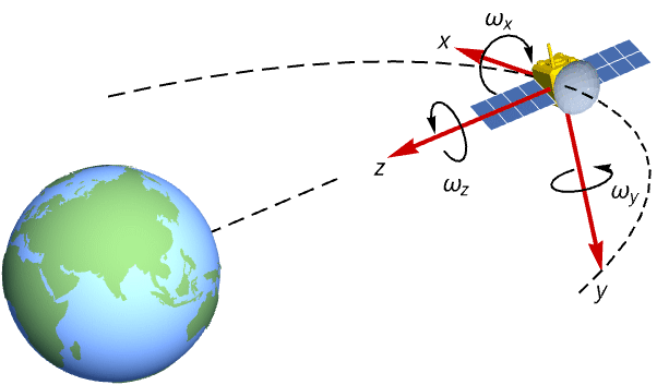
eqns = Table[Subscript[j, i[[1]]] Subscript[ω, i[[1]]]'[t] - (Subscript[j, i[[2]]] - Subscript[j, i[[3]]])Subscript[ω, i[[2]]][t]Subscript[ω, i[[3]]][t] == Subscript[τ, i[[1]]][t], {i, {{x, y, z}, {y, z, x}, {z, x, y}}}] /. {Subscript[j, x] -> 300, Subscript[j, y] -> 320, Subscript[j, z] -> 270}

, , の固定値について方程式の安定性を解析する：

Wolfram Language code:

DStabilityConditions[eqns /. {Subscript[τ, x][t] -> -27 / 400, Subscript[τ, y][t] -> 3 / 200, Subscript[τ, z][t] -> 1 / 50}, {Subscript[ω, x], Subscript[ω, y], Subscript[ω, z]}, t]

不動点を作用点として選択する：

Wolfram Language code:

opPt = {Subscript[ω, x0] -> (1/30Sqrt[3]), Subscript[ω, y0] -> (3Sqrt[3]/100), Subscript[ω, z0] -> (3Sqrt[3]/200), Subscript[τ, x0] -> -(27/400), Subscript[τ, y0] -> (3/200), Subscript[τ, z0] -> (1/50)};

状態空間モデルを構築する：

Wolfram Language code:

ssm = StateSpaceModel[eqns, {{Subscript[ω, x][t], Subscript[ω, x0]}, {Subscript[ω, y][t], Subscript[ω, y0]}, {Subscript[ω, z][t], Subscript[ω, z0]}}, {{Subscript[τ, x][t], Subscript[τ, x0]}, {Subscript[τ, y][t], Subscript[τ, y0]}, {Subscript[τ, z][t], Subscript[τ, z0]}}, {Subscript[ω, x][t], Subscript[ω, y][t], Subscript[ω, z][t]}, t, SystemsModelLabels -> {{Subscript[τ, x], Subscript[τ, y], Subscript[τ, z]}, {Subscript[ω, x], Subscript[ω, y], Subscript[ω, z]}, {Subscript[ω, x], Subscript[ω, y], Subscript[ω, z]}}] /. opPt

衛星の姿勢は，妨害されると調整できない：

Wolfram Language code:

OutputResponse[{ssm, {0.2, -0.1, 0.35}}, {0, 0, 0}, {t, 0, 3000}];
Plot[%, {t, 0, 3000}, PlotRange -> All, PlotLegends -> {Subscript[ω, x], Subscript[ω, y], Subscript[ω, z]}]

モデルの可制御性を検証する：

Wolfram Language code: ControllableModelQ[ssm]

ラグランジュ(Lagrangian)を使って倒立振子について調べる：

の位置：

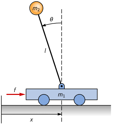
Wolfram Language code: Subscript[r, p] = Composition[TranslationTransform[{x[t], 0, 0}], RotationTransform[θ[t], {0, 0, 1}]][{0, 1, 0}]

速度：

Wolfram Language code: Subscript[v, p] = D[Subscript[r, p], t]

台車と振子の運動エネルギー：

Wolfram Language code: 𝒦 = (1/2)Subscript[m, 1] x'[t]^2 + (1/2)Subscript[m, 2]Subscript[v, p].Subscript[v, p]

振子の位置エネルギー：

Wolfram Language code: 𝒰 = Subscript[m, 2]g Subscript[r, p][[2]]

ラグランジュ：

Wolfram Language code: ℒ = 𝒦 - 𝒰

一般化された力：

Wolfram Language code: {Subscript[f, x], Subscript[f, θ]} = D[f[t] δx - Subscript[b, x]x'[t]δx - Subscript[b, θ]θ'[t]δθ, {{δx, δθ}}]

運動方程式：

Wolfram Language code: eqns = Table[Subscript[∂, t]D[ℒ, q'[t]] - D[ℒ, q[t]] == Subscript[f, q], {q, {x, θ}}]//Simplify

状態空間モデル：

Wolfram Language code:

ssm = StateSpaceModel[eqns, {x[t], x'[t], θ[t], θ'[t]}, f[t], {x[t], θ[t]}, t, SystemsModelLabels -> {f, {x, θ}, {x, Derivative[1][x], θ, Derivative[1][θ]}}]

非正の固有値で系は不安定になる：

Wolfram Language code:

Eigenvalues[First[Normal[ssm /. {Subscript[m, 1] -> 1 / 2, Subscript[m, 2] -> 1 / 10, l -> 3 / 10, g -> 10, Subscript[b, x] -> 15 / 100, Subscript[b, θ] -> 1 / 100}]]]//N

Wolfram Language code:

DFixedPoints[eqns /. {Subscript[m, 1] -> 1 / 2, Subscript[m, 2] -> 1 / 10, l -> 3 / 10, g -> 10, Subscript[b, x] -> 15 / 100, Subscript[b, θ] -> 1 / 100, f[t] -> 0}, {x, θ}, t]

Wolfram Language code:

DStabilityConditions[eqns /. {Subscript[m, 1] -> 1 / 2, Subscript[m, 2] -> 1 / 10, l -> 3 / 10, g -> 10, Subscript[b, x] -> 15 / 100, Subscript[b, θ] -> 1 / 100, f[t] -> 0}, {x, θ}, t, {{1, 0, 2Pi, 0}, {1, 0, 3Pi, 0}}]

特性と関係 (9)

DStabilityConditionsは，微分方程式の不動点と安定性条件を返す：

Wolfram Language code: DStabilityConditions[y'[t] == a y[t], y, t]

Wolfram Language code: DStabilityConditions[y'[t] == (1/2)y[t], y, t]

Wolfram Language code: DStabilityConditions[y'[t] == -(1/2) y[t], y, t]

DFixedPointsを使って微分方程式のすべての不動点を求める：

Wolfram Language code: DFixedPoints[y'[t] == 2 y[t](1 - y[t]), y[t], t]

特定の不動点における安定性を解析する：

Wolfram Language code: DStabilityConditions[y'[t] == 2 y[t](1 - y[t]), y[t], t, {{0}}]

Wolfram Language code: DStabilityConditions[y'[t] == 2 y[t](1 - y[t]), y[t], t, {{1}}]

DFixedPointsを使って非線形常微分方程式のすべての不動点を求める：

Wolfram Language code: points = DFixedPoints[x'[t] == x[t]^2 + 3x[t], x, t]

Solveを使って不動点を求める：

Wolfram Language code: Solve[x^2 + 3x == 0, x]

最初の不動点近くで方程式を線形化する：

Wolfram Language code:

f1 = D[x^2 + 3x, x] /. x -> points[[1, 1]];
leqn1 = x'[t] == f1 x[t]

最初の不動点近くでの安定性をチェックする：

Wolfram Language code: DStabilityConditions[leqn1, x, t][[1, 2]]

2番目の不動点近くで方程式を線形化する：

Wolfram Language code:

f1 = D[x^2 + 3x, x] /. x -> points[[2, 1]];
leqn2 = x'[t] == f1 x[t]

2番目の不動点近くの安定性をチェックする：

Wolfram Language code: DStabilityConditions[leqn2, x, t][[1, 2]]

DStabilityConditionsを使って非線形方程式の安定性を判定する：

Wolfram Language code: DStabilityConditions[x'[t] == x[t]^2 + 3x[t], x, t]

n 次微分方程式の不動点は， n 次元ベクトルである：

Wolfram Language code: DStabilityConditions[y''[t] + y'[t] + 3 y[t] == 5, y, t]

n 個の一次微分方程式の系の不動点は，n 次元ベクトルである：

Wolfram Language code: DStabilityConditions[{y'[t] + z[t] == 3, y[t] + 2 z'[t] == 1}, {y[t], z[t]}, t]

2つの常微分方程式の系の安定性を解析する：

Wolfram Language code: DStabilityConditions[{x'[t] == -x[t] - y[t] - 1, y'[t] == 2x[t] - y[t] + 5}, {x, y}, t]

不動点を初期条件として使って，DSolveValueで系を解く：

Wolfram Language code:

sol = DSolveValue[{x'[t] == -x[t] - y[t] - 1, y'[t] == 2x[t] - y[t] + 5, x[0] == -2, y[0] == 1}, {x[t], y[t]}, t]//Simplify

与えられた初期条件についてDSolveValueを使って系を解く：

Wolfram Language code:

sol = DSolveValue[{x'[t] == -x[t] - y[t] - 1, y'[t] == 2x[t] - y[t] + 5, x[0] == 3, y[0] == -2}, {x[t], y[t]}, t]//Simplify

解をプロットする：

Wolfram Language code: Plot[Evaluate[sol], {t, 0, 20}]

非線形常微分方程式の安定性を解析する：

Wolfram Language code: DStabilityConditions[x'[t] == (1/2)x[t](1 - x[t]), x, t]

NDSolveを使って常微分方程式を解く：

Wolfram Language code: sol = NDSolve[{x'[t] == (1/2)x[t](1 - x[t]), x[0] == 0.5}, x[t], {t, 0, 20}]

解をプロットする：

Wolfram Language code: Plot[x[t] /. sol, {t, 0, 20}, PlotRange -> All]

非線形常微分方程式の安定性を解析する：

Wolfram Language code: DStabilityConditions[2 y'[x] - y[x] ^ 2 == -1, y, x]

最初の不動点を初期条件として使って常微分方程式の漸近解を計算する：

Wolfram Language code: AsymptoticDSolveValue[{2 y'[x] - y[x] ^ 2 == -1, y[0] == -1}, y, {x, 0, 6}]

別の初期条件についての常微分方程式の漸近解を計算する：

Wolfram Language code: AsymptoticDSolveValue[{2 y'[t] - y[t] ^ 2 == -1, y[0] == -1 + ϵ}, y, t, {ϵ, 0, 2}]

Wolfram Language code: Limit[%, t -> Infinity]

Wolfram Language code: AsymptoticDSolveValue[{2 y'[t] - y[t] ^ 2 == -1, y[0] == 1 + ϵ}, y, t, {ϵ, 0, 2}]

Wolfram Language code: Limit[%, t -> Infinity, Assumptions -> Im[ϵ] == 0]

2つの非線形常微分方程式の系の不動点を求める：

Wolfram Language code: points = DFixedPoints[{x'[t] == x[t](2−x[t]−y[t]), y'[t] == −x[t] + 3y[t]−2x[t] y[t]}, {x, y}, t]

系のヤコビ行列を計算する：

Wolfram Language code: (jacobian = D[{x(2−x−y), −x + 3y−2x y}, {{x, y}}])//MatrixForm

各不動点についてヤコビ行列の固有値を計算する：

Wolfram Language code: eig1 = Eigenvalues[jacobian /. Thread[{x, y} -> points[[1]]]]

Wolfram Language code: eig2 = Eigenvalues[jacobian /. Thread[{x, y} -> points[[2]]]]

Wolfram Language code: eig3 = Eigenvalues[jacobian /. Thread[{x, y} -> points[[3]]]]

すべての固有値が負の実部を持つなら，この系は不動点近くで局所的に安定している：

Wolfram Language code: Re[#] < 0& /@ eig1

Wolfram Language code: Re[#] < 0& /@ eig2

Wolfram Language code: Re[#] < 0& /@ eig3

DStabilityConditionsを使って点の安定性をチェックする：

Wolfram Language code: DStabilityConditions[{x'[t] == x[t](2−x[t]−y[t]), y'[t] == −x[t] + 3y[t]−2x[t] y[t]}, {x, y}, t]

考えられる問題 (2)

場合によっては，安定性の条件が最も単純ではないことがある：

Wolfram Language code:

res = DStabilityConditions[{σ(−x[t] + y[t]) == x'[t], r x[t]−y[t]−x[t] z[t] == y'[t], −b z[t] + x[t] y[t] == z'[t]}, {x, y, z}, t]

さらに処理することでもっと簡約することができる：

Wolfram Language code: Simplify[#, b > 0 && r > 1 && σ > 0]& /@ res

与えられた点が混合整数ではないので，DStabilityConditionsはうまくいかない：

Wolfram Language code: DStabilityConditions[y'[t] == y[t](1 - y[t]), y, t, {{2}}]

まず，DFixedPoints を使って方程式のすべての不動点を求める：

Wolfram Language code: points = DFixedPoints[y'[t] == 3 y[t](1 - y[t]), y, t]

Wolfram Language code: DStabilityConditions[y'[t] == 3 y[t](1 - y[t]), y, t, {points[[1]]}]

Wolfram Language code: DStabilityConditions[y'[t] == 3 y[t](1 - y[t]), y, t, {points[[2]]}]

おもしろい例題 (2)

van der Pol振動子は，非保存的な，非線形減衰がある振動する系である：

Wolfram Language code: sys = {x'[t] == y[t], y'[t] == -x[t] + μ (1 - x[t]^2)y[t]};

系の安定性を解析する：

Wolfram Language code: DStabilityConditions[sys, {x, y}, t]

パラメータのさまざまな値について，系の軌道をアニメーション化する：

Wolfram Language code: Animate[StreamPlot[{y, -x + μ (1 - x^2)y}, {x, -4, 4}, {y, -4, 4}], {μ, 0.01, 4}]

FitzHugh–Nagumoモデルは弛緩振動子の例である：

Wolfram Language code: sys = {x'[t] == 3y[t] - x[t](x[t]^2 - 3) + s, y'[t] == (7 - 10x[t] - 8y[t]) / 30};

外部からの刺激 s が特定の閾値を超えると，系は変数 x および y が弛緩して静止値に戻る前に位相空間における特徴的な偏位を示す：

Wolfram Language code: DStabilityConditions[sys /. s -> 1 / 100, {x, y}, t]

パラメータ s のさまざまな値について系の軌跡を可視化する：

Wolfram Language code: Animate[StreamPlot[{3y - x(x^2 - 3) + s, (7 - 10x - 8y) / 30}, {x, -3, 3}, {y, -3, 3}], {s, 0.01, 4}]

Top

その他のラーニングリソース

テクニカルサポート

データサイエンス，金融，ビジネス

工学

科学とテクノロジー

教育のためのテクノロジー

教育イニシアチブ

使い始める

Grow Your Skills

Wolframと繋がる

大人用の教育プログラム

若者のための教育プログラム

読む

DStabilityConditions

詳細とオプション

例題

例 (5)

スコープ (25)

線形方程式 (5)

非線形方程式 (3)

線形系 (12)

非線形系 (5)

オプション (2)

Assumptions (2)

アプリケーション (11)

物理学 (5)

生物学 (3)

化学 (1)

制御系 (2)

特性と関係 (9)

考えられる問題 (2)

おもしろい例題 (2)

テキスト

CMS

APA

BibTeX

BibLaTeX

DStabilityConditions

詳細とオプション

例題

例 (5)

スコープ (25)

線形方程式 (5)

非線形方程式 (3)

線形系 (12)

非線形系 (5)

オプション (2)

Assumptions (2)

アプリケーション (11)

物理学 (5)

生物学 (3)

化学 (1)

制御系 (2)

特性と関係 (9)

考えられる問題 (2)

おもしろい例題 (2)

関連項目

関連するガイド

履歴

テキスト

CMS

APA

BibTeX

BibLaTeX