DiscreteMaxLimit[f,k∞]
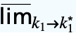
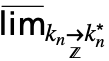
给出序列 f[k] 当 k 在整数上趋近于 ∞ 时的最大极限 k∞f(k).
DiscreteMaxLimit[f,{k1
,…,kn
}]
给出整数上的嵌套最大极限
⋯
f(k1,…,kn).
DiscreteMaxLimit[f,{k1,…,kn}{
,…,
}]
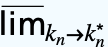
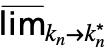
给出整数上的多变量最大极限
f(k1,…,kn).
DiscreteMaxLimit
DiscreteMaxLimit[f,k∞]
给出序列 f[k] 当 k 在整数上趋近于 ∞ 时的最大极限 k∞f(k).
DiscreteMaxLimit[f,{k1
,…,kn
}]
给出整数上的嵌套最大极限
⋯
f(k1,…,kn).
DiscreteMaxLimit[f,{k1,…,kn}{
,…,
}]
给出整数上的多变量最大极限
f(k1,…,kn).
更多信息和选项
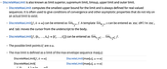
- DiscreteMaxLimit 亦称为 limit superior、supremum limit、limsup、upper limit 和 outer limit.
- DiscreteMaxLimit 计算极限的最小上限,且总是为实值序列定义. 它通常用于给出不依赖于实际极限的收敛条件和其他渐进属性.
- 可用
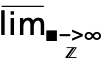
f 来输入 DiscreteMaxLimit[f,k∞]. 可用
dMlim
来输入模板
,用
把光标从底部移动到主体. - 可用
…
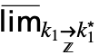
f 来输入 DiscreteMaxLimit[f,{k1,…,kn}{
,…,
}].
的极限值为 ±∞. - 最大极限被定义为最大包络序列 max[ω] 的极限:
-
DiscreteMaxLimit[f,k∞] DiscreteLimit[max[ω],ω∞] DiscreteMaxLimit[f,{k1,…,kn}{∞,…,∞}] DiscreteLimit[max[ω],ω∞] - DiscreteMaxLimit[f[k],k-∞] 等价于 DiscreteMaxLimit[f[-l],l∞] 等.
- 对单变量 f[k],定义使用最大包络 max[ω]MaxValue[{f[k],k≥ω∧k∈
},k],对多变量 f[k1,…,kn],则使用 max[ω]MaxValue[{f[k1,…,kn],k1≥ω∧⋯∧kn≥ω∧ki∈
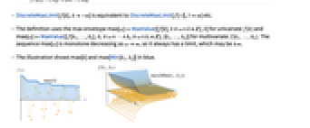
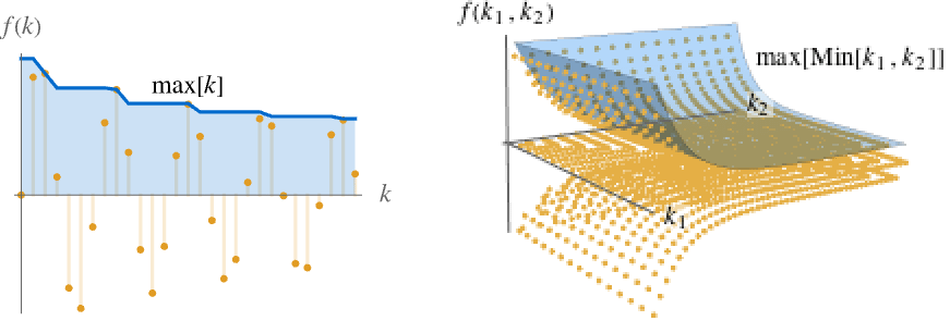
},{k1,…,kn}]. ω∞ 时,序列 max[ω] 单调递减,所以它总是有一个极限,可能是 ±∞. - 下图中用蓝色显示 max[k] 和 max[Min[k1,k2]].
- 如果无法找到最大极限,DiscreteMaxLimit 不进行计算,直接返回.
- 可以给出下列选项:
-
Assumptions $Assumptions 对参数的假设 GenerateConditions Automatic 是否为参数生成条件 Method Automatic 所用的方法 PerformanceGoal "Quality" 优化的目标 - GenerateConditions 的可能设置包括:
-
Automatic 只汇报非通用条件 True 汇报所有条件 False 不汇报条件 None 如果需要条件,则不进行计算,直接返回 - PerformanceGoal 的可能设置包括 $PerformanceGoal、"Quality" 和 "Speed". 如果设置为 "Quality", DiscreteMaxLimit 通常能求解更多问题或产生更简单的结果,但会需要更多时间和内存.
范例
打开所有单元 关闭所有单元基本范例 (4)
DiscreteMaxLimit[(-1) ^ n, n -> ∞]DiscretePlot[{(3 + (24 / 25) ^ n) Sin[Pi(n / 20)]}, {n, 1, 200, 3}, PlotRange -> {-4, 4}]DiscreteMaxLimit[(3 + (24 / 25) ^ n) * Sin[Pi(n / 20)], n -> ∞]用
dMlim
输入模板
, 用
把光标从底部移动到主体:
Underscript[, nUnderscript[ -> , ℤ]∞]Sin[n]TraditionalForm 输出:
DiscreteMaxLimit[f[n], n -> Infinity]//TraditionalForm范围 (21)
基本用法 (4)
计算当 n 趋近于 Infinity 时序列的最大极限:
DiscreteMaxLimit[(-1) ^ n 3n ^ 2 / (n ^ 2 + 5), n -> ∞]计算当 n 趋近于 -Infinity 时序列的最大极限:
DiscreteMaxLimit[Sin[n π / 2](5 + 3 ^ n), n -> -∞]DiscreteMaxLimit[Cos[m + 1 / (n + 1)], {m -> ∞, n -> ∞}]DiscreteMaxLimit[{(2) ^ (-n), Cos[n π]}, n -> ∞]初等函数序列 (6)
DiscreteMaxLimit[(-1) ^ n(3n) / (1 + 6n), n -> ∞]DiscretePlot[{(-1) ^ n(3n) / (1 + 6n), 1 / 2}, {n, 0, 50}]DiscreteMaxLimit[(-9 / 10) ^ n, n -> ∞]DiscretePlot[{(-9 / 10) ^ n}, {n, 10, 40}]DiscreteMaxLimit[(-1) ^ n, n -> ∞]DiscretePlot[{(-1) ^ n}, {n, 10, 30}]DiscreteMaxLimit[(-3) ^ n, n -> ∞]DiscretePlot[{(-10 / 9) ^ n}, {n, 10, 50}]DiscreteMaxLimit[E ^ ((-1) ^ n(n) / (n + 2)), n -> ∞]DiscretePlot[{E ^ ((-1) ^ n(n) / (n + 2)), E}, {n, 1, 50}]DiscreteMaxLimit[2 ^ Sin[n], n -> ∞]DiscretePlot[{2 ^ Sin[n], 2}, {n, 1, 50}]DiscreteMaxLimit[Sin[n], n -> ∞]DiscretePlot[{Sin[n], 1}, {n, 1, 150}]DiscreteMaxLimit[(3n / (n + 1) + (14 / 17) ^ n)Cos[Pi(n / 20)], n -> ∞]DiscretePlot[{(3 n / (n + 1) + (14 / 17) ^ n) * Cos[Pi(n / 20)], 3}, {n, 1, 200, 3}, PlotRange -> {-4, 4}]DiscreteMaxLimit[(-1) ^ n ArcTan[n], n -> ∞]DiscretePlot[{(-1) ^ n ArcTan[n], Pi / 2}, {n, 1, 30}]DiscreteMaxLimit[Log[1 + n / (n + 1)] Sin[n Pi / 5], n -> ∞]DiscretePlot[{Log[1 + n / (n + 1)] Sin[n Pi / 5], %}, {n, 1, 50}]周期序列 (3)
DiscreteMaxLimit[Mod[n, 5], n -> ∞]DiscretePlot[Mod[n, 5], {n, 1, 20}]DiscreteMaxLimit[Sin[n Pi / 4], n -> ∞]DiscretePlot[Sin[n Pi / 4], {n, 1, 40}]DiscreteMaxLimit[Cos[Pi n / 10], n -> ∞]DiscretePlot[Cos[Pi n / 10], {n, 1, 20}]Table[Mod[Factorial[n] + (-1) ^ n, 5], {n, 12}]DiscreteMaxLimit[Mod[Factorial[n] + (-1) ^ n, 5], n -> ∞]DiscretePlot[Mod[Factorial[n] + (-1) ^ n, 5], {n, 1, 20}]DiscreteMaxLimit[Sin[n], n -> ∞]DiscretePlot[{Sin[n], 1}, {n, 1, 150}]DiscreteMaxLimit[Exp[Sin[2n] ^ 2 / (2 + Cos[n])], n -> ∞]N[%]DiscretePlot[Exp[Sin[2n] ^ 2 / (2 + Cos[n])], {n, 1, 150}]分段序列 (2)
DiscreteMaxLimit[Piecewise[{{n, n ≤ 4}}, Sin[n]], n -> ∞]DiscretePlot[{Piecewise[{{n, n ≤ 4}}, Sin[n] ], 1}, {n, 0, 75}]DiscreteMaxLimit[Piecewise[{{Sin[n], n ≤ 10}}, n(-1) ^ n], n -> ∞]DiscretePlot[Piecewise[{{Sin[n], n ≤ 20}}, n(-1) ^ n], {n, 0, 75}]DiscreteMaxLimit[Piecewise[{{1 + 1 / n, Mod[n, 2] == 0}, {-1 - 1 / n, Mod[n, 2] == 1}}], n -> ∞]DiscretePlot[Piecewise[{{1 + 1 / n, Mod[n, 2] == 0}, {-1 - 1 / n, Mod[n, 2] == 1}}], {n, 1, 75}]特殊函数序列 (2)
计算涉及 Fibonacci 的序列的极限:
DiscreteMaxLimit[Fibonacci[n]Sin[n Pi / 2] / GoldenRatio ^ n, n -> ∞]涉及 FactorialPower 的序列:
DiscreteMaxLimit[(-1) ^ n(FactorialPower[n, 2] / (7n ^ 2 + 1)), n -> ∞]数论函数序列 (2)
DiscreteMaxLimit[LCM[Mod[n, 3], 20], n -> ∞]DiscreteMaxLimit[GCD[Mod[n, 56], 33], n -> ∞]涉及 Prime 的序列:
DiscreteMaxLimit[(-1) ^ n Prime[n] / (n Log[n]), n -> ∞]DiscretePlot[(-1) ^ n Prime[n] / (n Log[n]), {n, 10, 100}]多变量序列 (2)
DiscreteMaxLimit[(-1) ^ (m + n) (1000) ^ (1 / n) (m ^ 2 / (m ^ 2 + 1)), {m -> ∞, n -> ∞}]DiscretePlot3D[{(-1) ^ (m + n)(1000) ^ (1 / n)(m ^ 2 / (m ^ 2 + 1)), 1}, {n, 50, 60}, {m, 50, 60}, Filling -> None]DiscreteMaxLimit[(m + n/m n), {m, n} -> {∞, ∞}]DiscreteMaxLimit[Sin[(π n/3)]Cos[(π m/4)], {m, n} -> {∞, ∞}]选项 (6)
Assumptions (1)
GenerateConditions (3)
DiscreteMaxLimit[(1/2 + ^ n), n -> ∞, GenerateConditions -> False]DiscreteMaxLimit[(1/2 + ^ n), n -> ∞]DiscreteMaxLimit[Exp[a n]Sin[n], n -> ∞, GenerateConditions -> None]DiscreteMaxLimit[Exp[a n] Sin[n], n -> ∞]DiscreteMaxLimit[(x y/x^2 + (-1 + a x)^2 y^2), {x, y} -> {∞, ∞}]当设置为 GenerateConditions->True 时,即便是非通用条件,也会汇报:
DiscreteMaxLimit[(x y/x^2 + (-1 + a x)^2 y^2), {x, y} -> {∞, ∞}, GenerateConditions -> True]Method (1)
PerformanceGoal (1)
DiscreteMaxLimit 计算周期为任意长度的序列的极限:
expr = 1 / (Mod[n, 31] + 1 / (7 + Mod[n, 10 ^ 5]));DiscreteMaxLimit[expr, n -> ∞]用 PerformanceGoal 来避免此种花费时间较长的计算:
DiscreteMaxLimit[expr, n -> ∞, PerformanceGoal -> "Speed"]Method 选项会覆盖 PerformanceGoal:
DiscreteMaxLimit[expr, n -> ∞, Method -> "Periodic", PerformanceGoal -> "Speed"]应用 (7)
基本应用 (2)
DiscreteMaxLimit[(-1) ^ n E ^ (-10 / n), n -> ∞]DiscretePlot[{(-1) ^ n E ^ (-10 / n), 1}, {n, 1, 100}]a[n_] := n Sin[5n] / (3n + 1)DiscretePlot[a[n], {n, 1, 140}]证明 DiscreteMaxLimit 和 DiscreteMinLimit 不相等:
DiscreteMaxLimit[a[n], n -> ∞]DiscreteMinLimit[a[n], n -> ∞]用 DiscreteLimit 确认极限不存在:
DiscreteLimit[a[n], n -> ∞]级数收敛 (4)
a[n_] := Inactive[Product][1 / 2 (Mod[k, 2] + 1 / 5), {k, 1, n}]DiscretePlot[Activate[Sum[a[p], {p, 1, n}]], {n, 1, 20}]用 DiscreteRatio 计算相邻项的比:
rat = DiscreteRatio[a[n], n]Table[rat, {n, 1, 10}]DiscreteLimit[rat, n -> ∞]DiscreteMaxLimit[rat, n -> ∞]用 SumConvergence 确认级数是收敛的:
SumConvergence[a[p]//Activate, p]Sum[a[p]//Activate, {p, 1, ∞}]N[%]a[n_] := (2 / 3) ^ n Mod[n, 2]DiscretePlot[Activate[Sum[a[p], {p, 1, n}]], {n, 1, 20}, PlotRange -> {0.1, 1.2}]root = a[n] ^ (1 / n)Table[root, {n, 1, 20}]DiscreteLimit[root, n -> ∞]DiscreteMaxLimit[root, n -> ∞]用 SumConvergence 确认级数是收敛的:
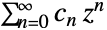
SumConvergence[a[p]//Activate, p]Sum[a[n]//Activate, {n, 1, ∞}]c[n_] := (Mod[n, 2]/n!)DiscreteMaxLimit[c[n]^(1/(n)), n -> ∞]FullSimplify[Underoverscript[∑, n = 0, ∞] (Mod[n, 2]/n!)z^n]f[z_] := (1/z^2 + 2)a[n_] = FullSimplify[(1/n!)D[f[z], {z, n}] /. z -> 0]Underoverscript[∑, n = 0, ∞]a[n]z^n == f[z]r = 1 / DiscreteMaxLimit[Abs[a[n]]^(1/(n)), n -> ∞]这表明泰勒级数对于距原点
的范围内的
值是收敛的. 例如,在
处:
Underoverscript[∑, n = 0, ∞]a[n]I^n == f[I]{Underscript[, k -> ∞]Underoverscript[∑, n = 0, k]a[n]2^n, Underscript[, k -> ∞]Underoverscript[∑, n = 0, k]a[n]2^n}Table[a[n](Sqrt[2])^n, {n, 0, 11}]Table[Underoverscript[∑, n = 0, k]a[n](Sqrt[2])^n, {k, 0, 11}]可视化
及其泰勒级数在
区间上的部分和;在区间内部,收敛是快速的,但泰勒多项式在端点处总是为
或
:
Plot[Evaluate@Prepend[Table[Underoverscript[∑, n = 0, k]a[n]x^n, {k, 0, 8, 2}], Style[f[x], AbsoluteThickness[2.5]]], {x, -Sqrt[2], Sqrt[2]}, PlotRange -> {0, .5}, PlotLegends -> "Expressions", PlotTheme -> "DashedLines"]计算复杂性 (1)
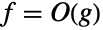
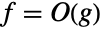
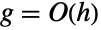
一个算法运行时间函数
被认为是 "big-o of
",写作
,如果
:
bigO[n_][f_, g_] := Underscript[, nUnderscript[ -> , ℤ]∞](f/g) < ∞同样,
还被认为是 "big-theta of
",写作
,如果
和
:
Θ[n_][f_, g_] := Underscript[, nUnderscript[ -> , ℤ]∞](f/g) < ∞ && Underscript[, nUnderscript[ -> , ℤ]∞](f/g) > 0bigO[n][f[n], f[n]]f = 10n ^ 2 + 2n + 1;
g = 5 n ^ 3;
h = n ^ 4 + 3n ^ 2 + 2;
{bigO[n][f, g], bigO[n][g, h], bigO[n][f, h]}f = 1;
g = (1/n)Mod[-1 + n, 2] + n Mod[n, 2];
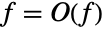
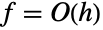
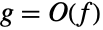
{bigO[n][f, g], bigO[n][g, f]}因此,
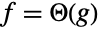
在算法运行时间空间 (runtime space) 上定义了自反部分关系,类似于
:
runtimes = {n ^ 2, 1, n, n Log[n], Exp[n]};Sort[runtimes, bigO[n]]f = 10n ^ 2 + 2n + 1;
g = 5 n ^ 2 + 100;
{bigO[n][f, g], bigO[n][g, f], Θ[n][f, g], Θ[n][g, f]}属性和关系 (11)
f[n_] := (-1) ^ nDiscreteMaxLimit[f[n], n -> ∞]DiscreteLimit[f[n], n -> ∞]f[n_] := Sin[n]g[n_] := Cos[n]DiscreteMaxLimit[f[n] + g[n], n -> ∞] <= DiscreteMaxLimit[f[n], n -> ∞] + DiscreteMaxLimit[g[n], n -> ∞]DiscreteMaxLimit[f[n] + g[n], n -> ∞] < DiscreteMaxLimit[f[n], n -> ∞] + DiscreteMaxLimit[g[n], n -> ∞]f[n_] := (-1) ^ nc = 6;DiscreteMaxLimit[c f[n], n -> ∞] == c DiscreteMaxLimit[f[n], n -> ∞]对于实值序列,如果 DiscreteLimit 存在,DiscreteMaxLimit 的值与之相等:
f[n_] := (-1) ^ n n / (n ^ 2 + 1)DiscreteLimit[f[n], n -> ∞]DiscreteMaxLimit[f[n], n -> ∞]f[n_] := n / (n + 1)g[n_] := Cos[n]DiscreteLimit[f[n], n -> ∞]DiscreteMaxLimit[f[n] + g[n], n -> ∞] == DiscreteMaxLimit[f[n], n -> ∞] + DiscreteMaxLimit[g[n], n -> ∞]DiscreteMaxLimit 总是大于或等于 DiscreteMinLimit:
f[n_] := Sin[n]DiscreteMinLimit[f[n], n -> ∞] ≤ DiscreteMaxLimit[f[n], n -> ∞]如果 DiscreteMaxLimit 等于 DiscreteMinLimit,极限存在并等于它们共有的值:
f[n_] := (n Cos[n]/n^2 + 1){Underscript[, nUnderscript[ -> , ℤ]∞]f[n], Underscript[, nUnderscript[ -> , ℤ]∞]f[n], Underscript[, nUnderscript[ -> , ℤ]∞]f[n]}f[n_] := -n^2{Underscript[, nUnderscript[ -> , ℤ]-∞]f[n], Underscript[, nUnderscript[ -> , ℤ]-∞]f[n], Underscript[, nUnderscript[ -> , ℤ]-∞]f[n]}可用 -DiscreteMinLimit[-f,…] 来计算 DiscreteMaxLimit:
f[n_] := Piecewise[{{n, Mod[n, 2] == 0}, {-1, True}}]DiscreteMaxLimit[f[x], x -> ∞] == -DiscreteMinLimit[-f[x], x -> ∞]f[n_] := Sin[n / 20] / ng[n_] := (-1/n)Reduce[f[n] ≥ g[n]n, Integers]//SimplifyUnderscript[, nUnderscript[ -> , ℤ]-∞]g[n] ≤ Underscript[, nUnderscript[ -> , ℤ]-∞]f[n] ≤ Underscript[, nUnderscript[ -> , ℤ]-∞]f[n]Underscript[, nUnderscript[ -> , ℤ]-∞]f[n] == Underscript[, nUnderscript[ -> , ℤ]-∞]g[n] == Underscript[, nUnderscript[ -> , ℤ]-∞]f[n]这是 "squeezing" 或 "sandwich" 定理的推广:
DiscretePlot[{f[x], g[x]}, {x, 500}, Filling -> {2 -> {1}}]MaxLimit 总是大于或等于 DiscreteMaxLimit:
g[n_] := Sin[n π + Pi / 4]DiscreteMaxLimit[g[n], n -> ∞]MaxLimit[g[n], n -> ∞]Show[Plot[{g[n], 1, 1 / Sqrt[2]}, {n, 0, 10}, PlotTheme -> "DashedLines"], DiscretePlot[g[n], {n, 0, 10}, PlotMarkers -> {"Point", Large}]]可能存在的问题 (1)
巧妙范例 (1)
f[n_] := {{Sin[n], 1}, {(-1) ^ n 3n ^ 2 / (n ^ 2 + 5), 3}, {(-1) ^ n, 1}, {(-1) ^ n E ^ (-10 / n), 1}, {n Sin[5n] / (3n + 1), 1 / 3}, {(-1.2) ^ n, 10000}}range = {{-1.1, 1.1}, {-3.1, 3.1}, {-1.1, 1.1}, {-1, 1}, {-0.36, 0.36}, {-1600, 1600}};Grid[Partition[Table[With[{r1 = f[n][[m, 1]], r2 = f[n][[m, 2]], r3 = range[[m]]},
DiscretePlot[{r1, r2}, {n, 1, 40}, PlotRange -> r3, ImageSize -> 210, PlotLabel -> Style[HoldForm[DiscreteMaxLimit[r1, n -> Infinity]] == DiscreteMaxLimit[f[n][[m, 1]], n -> Infinity], 13]]], {m, 1, 6}], 2], Frame -> All]文本
Wolfram Research (2017),DiscreteMaxLimit,Wolfram 语言函数,https://reference.wolfram.com/language/ref/DiscreteMaxLimit.html.
CMS
Wolfram 语言. 2017. "DiscreteMaxLimit." Wolfram 语言与系统参考资料中心. Wolfram Research. https://reference.wolfram.com/language/ref/DiscreteMaxLimit.html.
APA
Wolfram 语言. (2017). DiscreteMaxLimit. Wolfram 语言与系统参考资料中心. 追溯自 https://reference.wolfram.com/language/ref/DiscreteMaxLimit.html 年
BibTeX
@misc{reference.wolfram_2026_discretemaxlimit, author="Wolfram Research", title="{DiscreteMaxLimit}", year="2017", howpublished="\url{https://reference.wolfram.com/language/ref/DiscreteMaxLimit.html}", note=[Accessed: 15-September-2026]}
BibLaTeX
@online{reference.wolfram_2026_discretemaxlimit, organization={Wolfram Research}, title={DiscreteMaxLimit}, year={2017}, url={https://reference.wolfram.com/language/ref/DiscreteMaxLimit.html}, note=[Accessed: 15-September-2026]}