Wolfram Language & System Documentation Center

ElectrostaticPDEComponent

ElectrostaticPDEComponent[vars,pars]

yields an electrostatic PDE term with variables vars and parameters pars.

Details

ElectrostaticPDEComponent is typically used to generate an electrostatic equation with model variables vars and model parameters pars.
ElectrostaticPDEComponent returns a sum of differential operators to be used as a part of partial differential equations:

ElectrostaticPDEComponent models static electric fields produced by stationary charges in insulating, or dielectric materials.

ElectrostaticPDEComponent models electrostatic phenomena with the dependent variable , the electric scalar potential. is in units of volt [], independent variables in units of [].
Stationary variables vars are vars={V[x₁,…,x_n],{x₁,…,x_n}}.
ElectrostaticPDEComponent generally does not produces a time-dependent PDE.
ElectrostaticPDEComponent is based on a diffusion, a source and a derivative PDE term:

is the vacuum permittivity in units of [], the polarization vector in units of [ $TemplateBox[{InterpretationBox[, 1], {"C", , "/", , {"m", ^, 2}}, coulombs per meter squared, {{(, "Coulombs", )}, /, {(, {"Meters", ^, 2}, )}}}, QuantityTF]$ ] and the volume charge density in units of [ $TemplateBox[{InterpretationBox[, 1], {"C", , "/", , {"m", ^, 3}}, coulombs per meter cubed, {{(, "Coulombs", )}, /, {(, {"Meters", ^, 3}, )}}}, QuantityTF]$ ].
The polarization vector specifies the density of permanent or induced electric dipole moments inside a material.
The volume charge density models charge distributions, negative or positive.
ElectrostaticPDEComponent can produce different equations, depending on the constitutive relationship.
For linear materials, the ElectrostaticPDEComponent equation simplifies to:

is the unitless relative permittivity.
can be isotropic, orthotropic or anisotropic.
For nonlinear non-hysteresis ferroelectric materials, the ElectrostaticPDEComponent equation is given as:

is the remanent polarization vector in units of [ $TemplateBox[{InterpretationBox[, 1], {"C", , "/", , {"m", ^, 2}}, coulombs per meter squared, {{(, "Coulombs", )}, /, {(, {"Meters", ^, 2}, )}}}, QuantityTF]$ ].
The implicit default boundary condition for the electrostatic model is a 0 ElectricFluxDensityValue.
The units of the electrostatic model terms are in [ $TemplateBox[{InterpretationBox[, 1], {"C", , "/", , {"m", ^, 3}}, coulombs per meter cubed, {{(, "Coulombs", )}, /, {(, {"Meters", ^, 3}, )}}}, QuantityTF]$ ], or equivalently in [ $TemplateBox[{InterpretationBox[, 1], {"s", , "A", , "/", , {"m", ^, 3}}, second amperes per meter cubed, {{(, {"Amperes", , "Seconds"}, )}, /, {(, {"Meters", ^, 3}, )}}}, QuantityTF]$ ].
The following parameters pars can be given:

parameter	default	symbol
"Polarization"	{0,…}	, polarization vector in [ $TemplateBox[{InterpretationBox[, 1], {"C", , "/", , {"m", ^, 2}}, coulombs per meter squared, {{(, "Coulombs", )}, /, {(, {"Meters", ^, 2}, )}}}, QuantityTF]$ ]
"RegionSymmetry"	None
"RelativePermittivity"		, unitless relative permittivity
"RemanentPolarization"	{0,…}	, remanent polarization vector in [ $TemplateBox[{InterpretationBox[, 1], {"C", , "/", , {"m", ^, 2}}, coulombs per meter squared, {{(, "Coulombs", )}, /, {(, {"Meters", ^, 2}, )}}}, QuantityTF]$ ]
"Thickness"	1	, thickness in []
"CrossSectionalArea"	1	, cross-sectional area in [ $TemplateBox[{InterpretationBox[, 1], {{"m", ^, 2}}, meters squared, {"Meters", ^, 2}}, QuantityTF]$ ]
"VacuumPermittivity"		, vacuum permittivity in []
"VolumeChargeDensity"	0	, volume charge density in [ $TemplateBox[{InterpretationBox[, 1], {"C", , "/", , {"m", ^, 3}}, coulombs per meter cubed, {{(, "Coulombs", )}, /, {(, {"Meters", ^, 3}, )}}}, QuantityTF]$ ]

All parameters may depend on the spacial variable and dependent variable .
The number of independent variables determines the dimensions of or and the length of vectors and .
A possible choice for the parameter "RegionSymmetry" is "Axisymmetric".
"Axisymmetric" region symmetry represents a truncated cylindrical coordinate system where the cylindrical coordinates are reduced by removing the angle variable as follows:
dimension reduction equation

1D

2D
In 2D, when a "Thickness" is specified, the ElectrostaticPDEComponent equation is given as:

In 1D, when a "CrossSectionalArea" is specified, the ElectrostaticPDEComponent equation is given as:

In a 1D axisymmetric, when a "Thickness" is specified, the ElectrostaticPDEComponent equation is given as:

The input specification for the parameters is exactly the same as for their corresponding operator terms.
If no parameters are specified, the default electrostatic PDE is:

If the ElectrostaticPDEComponent depends on parameters that are specified in the association pars as …,keyp_i…,p_iv_i,…, the parameters are replaced with .

Examples

open all close all

Basic Examples (3)

Define an electrostatic model :

Set up an electrostatic model with particular material parameters:

Specify model variables and electrostatic parameters:

Set up and solve an electrostatic PDE:

Visualize the solution:

Scope (14)

1D (4)

Define a 1D electrostatic model with a cross-sectional area :

Model an electric potential field with two electric potential conditions at the sides.

Specify model variables and electrostatic parameters:

Set up and solve an electrostatic PDE:

Visualize the solution:

Model an electric potential field with two electric potential conditions at the sides and a discontinuous relative permittivity.

Specify model variables and electrostatic parameters:

Set up and solve an electrostatic PDE:

Visualize the solution:

2D (5)

Define a 2D electrostatic model with a polarization vector:

Define a 2D nonlinear electrostatic model with a remanent polarization vector:

Define a 2D electrostatic model with a thickness :

Define an orthotropic relative permittivity:

Define a fully anisotropic relative permittivity:

2D Axisymmetric (2)

Define a 2D axisymmetric electrostatic model:

Define a 2D axisymmetric orthotropic electrostatic model:

3D (1)

Model an electric potential field in a hollow ball with electric potential conditions at the inner and outer radii.

Specify model variables and electrostatic parameters:

Set up and solve an electrostatic PDE:

Visualize the solution:

Multi-material (2)

Set up an electrostatic model for several material regions:

Model an electric potential field with two electric potential conditions at the sides and a discontinuous relative permittivity.

Specify model variables and electrostatic parameters:

Set up and solve an electrostatic PDE:

Visualize the solution:

Applications (4)

1D (2)

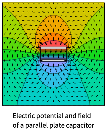
Compute the electric potential distribution between two parallel plates separated by a distance [] and positioned normal to the axis. The left plate is maintained at a constant potential [], whereas the right plate is grounded, []. The region between the plates is characterized by a relative permittivity and a uniform electron charge density [ $TemplateBox[{InterpretationBox[, 1], {"C", , "/", , {"m", ^, 3}}, coulombs per meter cubed, {{(, "Coulombs", )}, /, {(, {"Meters", ^, 3}, )}}}, QuantityTF]$ ]. The equation to model is given by:

Set up the electrostatic model variables :

Set up a region :

Specify electrostatic model parameters:

Specify the electric potential conditions:

Set up the equation:

Solve the PDE:

Visualize the solution:

Compute the electrical potential distribution between two parallel plates with the same distance and boundary conditions as in the previous example, but now with a nonuniform charge distribution given by:

Set up the electrostatic model variables :

Set up a region :

Specify electrostatic model parameters:

Specify the electric potential conditions:

Set up the equation:

Solve the PDE:

Visualize the solution:

2D (1)

Model an infinitely long rectangular box with metallic walls. The box has a width of [], and a height of []. The side and bottom walls are maintained at zero electric potential, whereas the top wall has a fixed electric potential of . The region inside the box is free of charge . The equation to model is given by:

Define the model variables and parameters:

Set up the model region:

Set up a 2D electrostatic model:

The side and bottom walls at , and are maintained at a zero electric potential:

The top wall at is fixed with an electric potential of []:

Set up the equation:

Solve the PDE:

Visualize the solution:

3D (1)

Model a dielectric material of a cylindrical capacitor with two electric potential conditions at the upper and lower boundaries, which represent the capacitor electrodes. The equation to model is given by:

Set up the electrostatic model variables :

Set up a region :

Specify a relative permittivity :

Specify ground potential at the lower boundary:

Specify an electric potential of [] at the upper boundary:

Set up the equation:

Solve the PDE:

Visualize the solution:

Possible Issues (1)

For symbolic computation, the "VacuumPermittivity" or "RelativePermittivity" parameter should be given as a matrix:

For numeric values, the "VacuumPermittivity" or "RelativePermittivity" parameter is automatically converted to a matrix of proper dimensions:

This automatic conversion is not possible for symbolic input:

Not providing the properly dimensioned matrix will result in an error:

Top

More Learning

Tech Support

Wolfram Solutions

Wolfram Solutions For Education

Get Started

Grow Your Skills

Work with Us

Educational Programs for Adults

Educational Programs for Youth

Read

ElectrostaticPDEComponent

Details

Examples

Basic Examples (3)