FunctionInjective[f,x]
![]() が各 y について最大1個の解 x∈Realsを持つかどうかを調べる.
が各 y について最大1個の解 x∈Realsを持つかどうかを調べる.
FunctionInjective[f,x,dom]
![]() が最大1個の解 x∈dom を持つかどうかを調べる.
が最大1個の解 x∈dom を持つかどうかを調べる.
FunctionInjective[{f1,f2,…},{x1,x2,…},dom]
![]() が最大1個の解 x1,x2,…∈dom を持つかどうかを調べる.
が最大1個の解 x1,x2,…∈dom を持つかどうかを調べる.
FunctionInjective[{funs,xcons,ycons},xvars,yvars,dom]
![]() が,条件 ycons で制約された各 yvars∈dom に対して条件 xcons で制約された最大1個の解 xvars∈dom を持つかどうかを調べる.
が,条件 ycons で制約された各 yvars∈dom に対して条件 xcons で制約された最大1個の解 xvars∈dom を持つかどうかを調べる.


FunctionInjective
FunctionInjective[f,x]
![]() が各 y について最大1個の解 x∈Realsを持つかどうかを調べる.
が各 y について最大1個の解 x∈Realsを持つかどうかを調べる.
FunctionInjective[f,x,dom]
![]() が最大1個の解 x∈dom を持つかどうかを調べる.
が最大1個の解 x∈dom を持つかどうかを調べる.
FunctionInjective[{f1,f2,…},{x1,x2,…},dom]
![]() が最大1個の解 x1,x2,…∈dom を持つかどうかを調べる.
が最大1個の解 x1,x2,…∈dom を持つかどうかを調べる.
FunctionInjective[{funs,xcons,ycons},xvars,yvars,dom]
![]() が,条件 ycons で制約された各 yvars∈dom に対して条件 xcons で制約された最大1個の解 xvars∈dom を持つかどうかを調べる.
が,条件 ycons で制約された各 yvars∈dom に対して条件 xcons で制約された最大1個の解 xvars∈dom を持つかどうかを調べる.
詳細とオプション
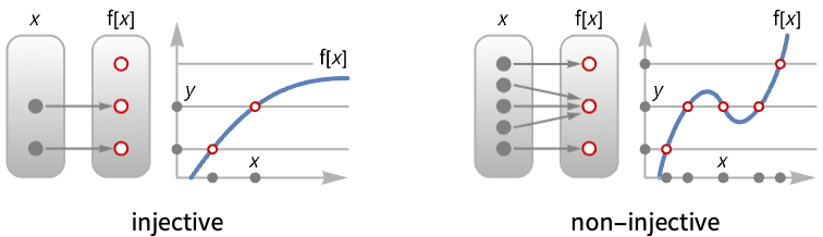
- 単射関数は一対一の関数としても知られている.
- 各
 に対して
に対して  となる最大で1つの
  がある場合,関数
  は単射である.
 - 写像
 が単射ならFunctionInjective[{funs,xcons,ycons},xvars,yvars,dom]はTrueを返す.ただし,
 は xcons の解集合で
  は ycons の解集合である.
 - funs が xvars 以外のパラメータを含むなら,結果は,一般に,ConditionalExpressionである.
- dom の可能な値にはRealsとComplexesがある.dom がRealsのときは,変数,パラメータ,定数,関数値がすべて実数でなければならない.
- funs の領域はFunctionDomainが与える条件によって制限される.
- xcons と ycons は,等式,不等式,あるいはそれらの論理結合を含むことができる.
- 次は,使用可能なオプションである,
-
Assumptions $Assumptions パラメータについての仮定 GenerateConditions True パラメータについての条件を生成するかどうか PerformanceGoal $PerformanceGoal 速度と品質のどちらを優先するか - 次は,GenerateConditionsの可能な設定である.
-
Automatic 一般的ではない条件のみ True すべての条件 False 条件なし None 条件が必要な場合は未評価で返す - PerformanceGoalの可能な値は"Speed"と"Quality"である.
例題
すべて開く すべて閉じる例 (4)
FunctionInjective[E ^ x, x]FunctionInjective[E ^ x, x, Complexes]FunctionInjective[{x + y ^ 3, y - x ^ 5}, {x, y}]FunctionInjective[x ^ 3 + a x + b, x]スコープ (13)
FunctionInjective[x ^ 3 - x, x]Plot[{x ^ 3 - x, 1 / 4}, {x, -2, 2}]FunctionInjective[{x ^ 3 - x, x > 1}, x]Plot[{x ^ 3 - x, 10}, {x, 1, 3}]FunctionInjective[{x ^ 3 - x, True, y > 1 / 2}, x, y]Plot[{x ^ 3 - x, 1 / 2}, {x, -2, 2}]FunctionInjective[Log[x], x, Complexes]Reduce[Log[x] == y, x]FunctionInjective[{x ^ 3, Re[x] ≥ 0 && Im[x] ≥ 0}, x, Complexes]FunctionInjective[x ^ 3, x, Complexes]Reduce[x ^ 3 == 1, x]FunctionInjective[{x ^ 2, Re[x] >= 0, Im[y] != 0}, x, y, Complexes]FunctionInjective[{x ^ 2, Re[x] >= 0}, x, y, Complexes]Reduce[x ^ 2 == -1 && Re[x] >= 0, x]FunctionInjective[{Sin[x], Element[x, Integers]}, x]A = {{1, 2, 3}, {4, 5, 6}, {7, 8, 9}};FunctionInjective[A.{x, y, z}, {x, y, z}]B = {{1, 2, 3}, {4, 5, 6}, {7, 8, 0}};FunctionInjective[B.{x, y, z}, {x, y, z}]線形写像は,その行列の階数が領域の次元と等しいときかつそのときに限り単射である:
{MatrixRank[A], MatrixRank[B]}FunctionInjective[{x ^ 2 + 2x, x ^ 3 - x}, x]ParametricPlot3D[{{x, x ^ 2 + 2x, x ^ 3 - x}, {x, 3, 0}}, {x, -3, 3}]FunctionInjective[{x ^ 2 + x, x ^ 3 - x}, x]ParametricPlot3D[{{x, x ^ 2 + x, x ^ 3 - x}, {x, 0, 0}}, {x, -2, 2}]FunctionInjective[{x ^ 3 - 3x y ^ 2, 3x ^ 2y - y ^ 3}, {x, y}]FunctionInjective[{{x ^ 3 - 3x y ^ 2, 3x ^ 2y - y ^ 3}, x ≥ 0 && y ≥ 0}, {x, y}]FunctionInjective[{x + y ^ 3, y - x ^ 5}, {x, y}, Complexes]Det[D[{x + y ^ 3, y - x ^ 5}, {{x, y}}]]Det[D[{x - (x + y / 27) ^ 3, y + (3 x + y / 9) ^ 3}, {{x, y}}]]FunctionInjective[{x - (x + y / 27) ^ 3, y + (3 x + y / 9) ^ 3}, {x, y}, Complexes]FunctionInjective[x ^ 3 + a x ^ 2 + b x + c, x]FunctionInjective[{x + a y ^ 3, y + b x ^ 3}, {x, y}]オプション (4)
Assumptions (1)
FunctionInjectiveは,任意の ![]() について
について ![]() の単射性を決定できない:
の単射性を決定できない:
FunctionInjective[BesselI[n, x], x]![]() が奇整数であると仮定するとFunctionInjectiveはうまくいく:
が奇整数であると仮定するとFunctionInjectiveはうまくいく:
FunctionInjective[BesselI[n, x], x, Assumptions -> Element[(n + 1) / 2, Integers]]Plot[Evaluate[Table[BesselI[n, x], {n, 1, 9, 2}]], {x, -10, 10}]GenerateConditions (2)
デフォルトで,FunctionInjectiveは記号パラメータについての条件を生成することがある:
FunctionInjective[E ^ x + a x, x]GenerateConditionsNoneとすると,FunctionInjectiveは条件付きの結果を与えることができない:
FunctionInjective[E ^ x + a x, x, GenerateConditions -> None]FunctionInjective[E ^ x + a x, x, GenerateConditions -> False]FunctionInjective[a x, x, Complexes]GenerateConditionsAutomaticのときは,一般的に真である条件は報告されない:
FunctionInjective[a x, x, Complexes, GenerateConditions -> Automatic]PerformanceGoal (1)
PerformanceGoalを使って潜在的に高くつく計算を回避する:
FunctionInjective[x ^ 5 + a x ^ 4 + b x ^ 3 + c x ^ 2 + d x, x, PerformanceGoal -> "Speed"]デフォルト設定は使用可能なあらゆるテクニックを使って結果を出そうとする:
FunctionInjective[x ^ 5 + a x ^ 4 + b x ^ 3 + c x ^ 2 + d x, x]アプリケーション (17)
基本的なアプリケーション (8)
FunctionInjective[Cos[x], x]Plot[{Cos[x], 1 / 2}, {x, -2Pi, 2Pi}]FunctionInjective[ArcTan[x], x]Plot[{ArcTan[x], 1, 2}, {x, -5, 5}]FunctionInjective[Sqrt[x], x]Plot[{Sqrt[x], 1, -1}, {x, -10, 10}]制限のない実部におけるClip[x]の単射性をチェックする:
FunctionInjective[Clip[x], x]値![]() と
と![]() は,それぞれ[-∞,-1]と[1, ∞]に複数回出現する:
は,それぞれ[-∞,-1]と[1, ∞]に複数回出現する:
Plot[Clip[x], {x, -2, 2}]区間[-1, 1]に制限されたClip[x]は単射である:
FunctionInjective[{Clip[x], -1 ≤ x ≤ 1}, x]任意の水平線がグラフと最大1回しか交差しない関数は単射である:
FunctionInjective[Erf[x], x]Manipulate[Plot[{Erf[x], a}, ...], {{a, 0.5}, -1.5, 1.5}]FunctionInjective[(3x ^ 3 + 7x ^ 2) / (2x ^ 3 + 1), x]Manipulate[Plot[{(3x ^ 3 + 7x ^ 2) / (2x ^ 3 + 1), a}, ...], {{a, 3}, -3, 4}]FunctionInjective[Tan[x], x]FunctionPeriodを使って関数が周期的かどうかをチェックする:
FunctionPeriod[Tan[x], x]Plot[{Tan[x], 1}, {x, -5 / 2Pi, 5 / 2Pi}]FunctionInjective[Sin[x] + 2x, x]FunctionSignを使って導関数の符号を求める:
FunctionSign[D[Sin[x] + 2x, x], x]Plot[Sin[x] + 2x, {x, -10, 10}]f = Integrate[Cos[t] ^ 2 + E ^ -t, {t, 0, x}]FunctionInjective[f, x]Plot[f, {x, 0, 10}]g = Integrate[TriangleWave[t] + 5 / 4, {t, 0, x}, Assumptions -> 0 ≤ x ≤ 2]FunctionInjective[{g, 0 ≤ x ≤ 2}, x]Plot[g, {x, 0, 2}]f = Piecewise[{{x, Sin[π x] ≥ 0}, {2Ceiling[x] - 1 - x, Sin[π x] < 0}}];FunctionInjective[{f, 0 < x < 10}, x]Plot[f, {x, 0, 10}, ImageSize -> Small]FunctionInjective[1 / x, x]Plot[1 / x, {x, -2, 2}]FunctionContinuous[{1 / x, x ≠ 0}, x]FunctionDomain[1 / x, x]FunctionInjective[{x^2 + y^2, x - y}, {x, y}]ParametricPlotの一部は2回変換されている:
ParametricPlot[{x^2 + y^2, x - y}, {x, -1, 1}, {y, 0, 1}, Mesh -> Full]FunctionInjective[{{x^2 + y^2, x - y}, x > 0 && y > 0}, {x, y}]ParametricPlotの各点は1回しかカバーされない:
ParametricPlot[{x^2 + y^2, x - y}, {x, 0, 1}, {y, 0, 1}, Mesh -> Full]ParametricPlot[{x^2 - y^2, x - y}, {x, -1, 1}, {y, -1, 1}, Mesh -> Full]Reduce[{x^2 - y^2, x - y} == {0, 0}, {x, y}]FunctionInjective[{{x^2 - y^2, x - y}, x ≠ y}, {x, y}]方程式と不等式を解く (4)
![]() の任意の値について方程式
の任意の値について方程式 ![]() が
が ![]() についての解を最大1個持つとき,
についての解を最大1個持つとき,![]() は単射である:
は単射である:
FunctionInjective[ArcTan[(x ^ 5 + 3x ^ 3 + 2x) / (4x ^ 4 + 4)], x]Plot[{ArcTan[(x ^ 5 + 3x ^ 3 + 2x) / (4x ^ 4 + 4)], 1, 2}, {x, -10, 10}]Solve[ArcTan[(x ^ 5 + 3x ^ 3 + 2x) / (4x ^ 4 + 4)] == 1, x, Reals]Solve[ArcTan[(x ^ 5 + 3x ^ 3 + 2x) / (4x ^ 4 + 4)] == 2, x, Reals]Solve[ArcTan[(x ^ 5 + 3x ^ 3 + 2x) / (4x ^ 4 + 4)] == y, x, Reals]f = {x ^ 3, x - y ^ 2}FunctionInjective[f, {x, y}]Solve[f == {2, 1}, {x, y}, Reals]FunctionInjective[{f, y ≥ 0}, {x, y}]Solve[f == {u, v} && y ≥ 0, {x, y}, Reals]f := Function[x, ConditionalExpression[Erf[x] ^ 3, Element[x, Reals]]]FunctionInjective[f[x], x]Plot[f[x], {x, -3, 3}]g = InverseFunction[f]Plot[g[y], {y, -1, 1}]連結集合上で定義される非零の微分を持つ微分可能な関数は単射である:
f = Log[x ^ 2 + 1]df = D[f, x]FunctionSign[{df, x > 0}, x]FunctionInjective[{f, x > 0}, x]invf = DSolveValue[{g'[y] == 1 / (df /. x -> g[y]), g[f /. x -> 1] == 1}, g[y], y]Simplify[{invf /. y -> f, f /. x -> invf}, x > 0 && Element[y, Reals]]確率と統計 (2)
pdf = PDF[NormalDistribution[], x]FunctionSign[pdf, x]Plot[pdf, {x, -5, 5}]cdf = CDF[NormalDistribution[], x]FunctionInjective[cdf, x]Plot[cdf, {x, -5, 5}]SurvivalFunctionとQuantileも単射である:
sf = SurvivalFunction[NormalDistribution[], x]FunctionInjective[sf, x]Plot[sf, {x, -5, 5}]qf = Quantile[NormalDistribution[], x]FunctionInjective[qf, x]Plot[qf, {x, 0, 1}]微積分 (3)
e = Exp[-(x ^ 3 + y ^ 2) ^ 2] / (y ^ 6 + 1)x ^ 2y ^ 2;f[{u_, v_}] := 1 / 9Exp[-u ^ 2] / (v ^ 2 + 1)
g = {x ^ 3 + y ^ 2, y ^ 3};FunctionInjective[g, {x, y}]f[g]Det[D[g, {{x, y}}]] === eFunctionRange[g, {x, y}, {u, v}]Integrate[f[{u, v}], {u, -Infinity, Infinity}, {v, -Infinity, Infinity}]Integrate[e, {x, -Infinity, Infinity}, {y, -Infinity, Infinity}]f = {(2 r (1 - t^2) u/(1 + t^2) (1 + u^2)), (4 r t u/(1 + t^2) (1 + u^2)), (r (1 - u^2)/1 + u^2)};ParametricPlot3D[Evaluate[f /. r -> 1], {t, -50, 50}, {u, 0, 50}, ...]FunctionInjective[{f, u > 0}, {t, u}, Assumptions -> r > 0]表面積は,![]() のグラム(Gram)行列式の平方根の積分と同じである:
のグラム(Gram)行列式の平方根の積分と同じである:
df = D[f, {{t, u}}];Integrate[Sqrt[Det[Transpose[df].df]], {u, 0, ∞}, {t, -∞, ∞}, Assumptions -> r > 0]f = {(4 (1 - t^2) u (1 - u^2)/(1 + t^2) (1 + u^2)^2), (8 t u (1 - u^2)/(1 + t^2) (1 + u^2)^2), (2 u/1 + u^2)};
g[{x_, y_, z_}] := E ^ (x + y + z)ParametricPlot3D[f, {t, 0, 50}, {u, -50, 50}, ...]FunctionInjective[{f, t > 0 && u ≠ 0 && t ^ 2 ≠ 1 && u ^ 2 ≠ 1}, {t, u}]df = D[f, {{t, u}}];NIntegrate[g[f]Sqrt[Det[Transpose[df].df]], {t, 0, ∞}, {u, -∞, ∞}]reg = ImplicitRegion[x ^ 2 + y ^ 2 - 4z ^ 2 + 4z ^ 4 == 0, {x, y, z}];NIntegrate[g[v], Element[v, reg]]特性と関係 (3)
![]() は,方程式
は,方程式 ![]() が各
が各 ![]() について最大1つの解を持つときかつそのときに限り単射である:
について最大1つの解を持つときかつそのときに限り単射である:
FunctionInjective[x ^ 2 + x + 1, x]FunctionInjective[x ^ 3 + x + 1, x]Solveを使って解を求める:
Solve[x ^ 2 + x + 1 == y, x, Reals]Solve[x ^ 3 + x + 1 == y, x, Reals]連結集合上の実数値の一変量連続関数は,単調であるときかつそのときに限り単射である:
FunctionInjective[{Sin[x], 0 ≤ x ≤ Pi}, x]FunctionInjective[{Cos[x], 0 ≤ x ≤ Pi}, x]Plot[{Sin[x], Cos[x]}, {x, 0, Pi}]FunctionMonotonicityを使って関数の単調性を決定する:
FunctionMonotonicity[{Sin[x], 0 ≤ x ≤ Pi}, x]FunctionMonotonicity[{Cos[x], 0 ≤ x ≤ Pi}, x]複素多項式写像は,逆多項式を持つときかつそのときに限り単射である:
F = {x - (x + y / 27) ^ 3, y + (3 x + y / 9) ^ 3};FunctionInjective[F, {x, y}, Complexes]Solveを使って逆多項式を求める:
G = {x, y} /. Solve[{u, v} == {x - (x + y / 27) ^ 3, y + (3 x + y / 9) ^ 3}, {x, y}][[1]]Expand[G /. Thread[{u, v} -> F]]Expand[F /. Thread[{x, y} -> G]]考えられる問題 (1)
FunctionInjectiveはFunctionDomainを使って関数の実領域を決定する:
FunctionInjective[Cosh[Sqrt[x]], x]![]() はFunctionDomainが報告した実領域において単射である:
はFunctionDomainが報告した実領域において単射である:
FunctionDomain[Cosh[Sqrt[x]], x]Plot[{Cosh[Sqrt[x]], 7}, {x, 0, 10}]Plot[{Cosh[Sqrt[x]], -1 / 2}, {x, -20, 10}]点が ![]() の実領域に属するためには,
の実領域に属するためには,![]() の部分式はすべて実数値でなければならない:
の部分式はすべて実数値でなければならない:
Refine[Element[Sqrt[x], Reals], x < 0]テキスト
Wolfram Research (2020), FunctionInjective, Wolfram言語関数, https://reference.wolfram.com/language/ref/FunctionInjective.html.
CMS
Wolfram Language. 2020. "FunctionInjective." Wolfram Language & System Documentation Center. Wolfram Research. https://reference.wolfram.com/language/ref/FunctionInjective.html.
APA
Wolfram Language. (2020). FunctionInjective. Wolfram Language & System Documentation Center. Retrieved from https://reference.wolfram.com/language/ref/FunctionInjective.html