Wolfram 语言与系统参考资料中心

GibbsPointProcess

GibbsPointProcess[{"PairPotential",μ, ϕ}, d]

表示中的密度为 μ、对势函数 (pair-potential function) 为 ϕ 的 Gibbs 点过程.

GibbsPointProcess[{"PairInteraction",μ, h}, d]

表示中密度为 μ、偶相互酌函数 (pair-interaction function) 为 h 的 Gibbs 点过程.

GibbsPointProcess[{"Papangelou",λ^*}, d]

表示中 Papangelou 条件密度为的 Gibbs 点过程.

GibbsPointProcess[{"Density",f}, d]

表示中密度函数与 f 成正比的 Gibbs 点过程.

GibbsPointProcess

GibbsPointProcess[{"PairPotential",μ, ϕ}, d]

表示中的密度为 μ、对势函数 (pair-potential function) 为 ϕ 的 Gibbs 点过程.

GibbsPointProcess[{"PairInteraction",μ, h}, d]

表示中密度为 μ、偶相互酌函数 (pair-interaction function) 为 h 的 Gibbs 点过程.

GibbsPointProcess[{"Papangelou",λ^*}, d]

表示中 Papangelou 条件密度为的 Gibbs 点过程.

GibbsPointProcess[{"Density",f}, d]

表示中密度函数与 f 成正比的 Gibbs 点过程.

更多信息

GibbsPointProcess 亦称为 Markov 点过程.
Gibbs 模型通常用于模拟点之间的相互作用，例如树木或植物争夺资源，相互排斥或吸引的粒子.
可用密度函数和径向对势函数或偶相互酌函数来指定只在成对的点之间有相互作用的 Gibbs 点过程.
密度函数是位置的非负函数，如果不存在点之间的相互作用，则模拟附近预期的点的数量.
对势函数是点之间距离的实函数；较大的值意味着不太可能找到彼此相距的两个点.
由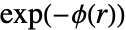给定的偶相互酌函数是点之间距离的非负函数；较大的值意味着比较有可能找到彼此相距的两个点.
GibbsPointProcess 可表示任意 Gibbs 点过程；常见的 Gibbs 过程都有专门实现的方法并且易于使用：

过程	对势	特点
HardcorePointProcess	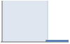	硬核相互作用
StraussPointProcess	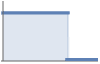	恒定强度的软核相互作用
StraussHardcorePointProcess	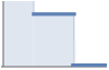	内部硬核，外层是软核
PenttinenPointProcess	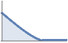	基于重叠区域大小的相互作用
DiggleGrattonPointProcess	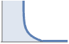	内部硬核，并带有递减软核
DiggleGatesPointProcess	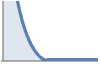	从硬核点平滑过渡

可用 Papangelou 密度或概率密度指定更广义的 Gibbs 点过程.
Papangelou 密度指定了将点添加到点集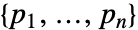内的成本，必须是非负函数.
密度指定了一个点布局的概率密度. 函数 f 必须是非负函数，但不必是归一化的.
GibbsPointProcess 允许 d 为任意正整数.
所有的指定都有一个等效的 Papangelou 密度 λ^*，如下所示：
{"PairPotential",μ,ϕ} $mu exp(-sum_iphi(TemplateBox[{{{p, _, i}, -, q}}, Norm]))$

{"PairInteraction",μ,h} $mu product_ip(TemplateBox[{{{p, _, i}, -, q}}, Norm])$ .

{"Density",f}
GibbsPointProcess 可与诸如 RipleyK 和 RandomPointConfiguration 这样的函数一起使用.

范例

打开所有单元关闭所有单元

基本范例 (1)

对具有适当密度函数的 GibbsPointProcess 给出的泊松点过程进行采样：

Wolfram Language code: h = Function[pts, 100 ^ Length[pts]];

Wolfram Language code: pts = RandomPointConfiguration[GibbsPointProcess[{"Density", h}, 2], Disk[]]

在区域上绘制点：

Wolfram Language code: Show[RegionPlot[pts["ObservationRegion"]], ListPlot[pts]]

范围 (4)

模拟密度与点数成正比的 Gibbs 点过程：

Wolfram Language code:

β = 30;
h = Function[pts, β ^ Length[pts]];

使用 Markov 链 Monte Carlo 方法模拟单位圆盘上的 40 个样本：

Wolfram Language code:

n = 40;
region = Disk[];

Wolfram Language code: sample = RandomPointConfiguration[GibbsPointProcess[h, 2], region, n, Method -> {"MCMC", "LengthOfRun" -> 10000}]

计算区域中的平均点数：

Wolfram Language code: Mean[sample["PointCountList"]]//N

与经过缩放的区域进行比较：

Wolfram Language code: val = β RegionMeasure[region]//N

Wolfram Language code: ListPlot[{sample["PointCountList"], {{0, val}, {n, val}}}, Joined -> {False, True}]

对 GibbsPointProcess 给出的 Strauss 点过程进行采样：

Wolfram Language code:

pairWiseDists[{}] := {}
pairWiseDists[pts_] := Block[{tp = pts}, Table[EuclideanDistance[pt, #]& /@ (tp = Rest[tp]), {pt, Most[pts]}]]

Wolfram Language code:

straussDensity[gamma_, beta_, R_] := Function[pts, Block[{dists, n = Length[pts]}, 
	dists = Total[Clip[Flatten[pairWiseDists[pts]], {0, R}, {0, 0}]];
	beta ^ n * gamma  ^ dists
	]
	];

Wolfram Language code: a = RandomPointConfiguration[GibbsPointProcess[straussDensity[.8, 30, 1], 2], Disk[], 1]

通过指定 Papangelou 条件密度对同一过程进行采样：

Wolfram Language code:

straussPapangelouDensity[gamma_, beta_, R_] := Function[{pts, newpt}, 
	beta * gamma  ^ Total[Clip[EuclideanDistance[newpt, #]& /@ pts, {0, R}, {0, 0}]]
	];

Wolfram Language code: b = RandomPointConfiguration[GibbsPointProcess[{"Papangelou", straussPapangelouDensity[.8, 30, 1]}, 2], Disk[], 1]

通过指定对势函数对同一过程进行采样：

Wolfram Language code: ϕ[γ_, R_] := Function[r, -Log[γ]Boole[r ≤ R]];

Wolfram Language code: c = RandomPointConfiguration[GibbsPointProcess[{"PairPotential", 30, ϕ[.8, 1]}, 2], Disk[], 1]

Wolfram Language code: Show[RegionPlot[Disk[]], ListPlot[#]]& /@ {a, b, c}

来自半径为 0.3 的硬核点过程的样本与密度为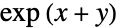的泊松点过程：

Wolfram Language code:

R = .3;
reg = Rectangle[{-3, -3}, {3, 3}];

Wolfram Language code:

μ = Exp[Total[#]]&;
	ϕ[R_] = Piecewise[{{∞, # < R}}]&;

Wolfram Language code: pts1 = RandomPointConfiguration[GibbsPointProcess[{"PairPotential", μ, ϕ[R]}, 2], reg]

Wolfram Language code: Show[RegionPlot[reg], ListPlot[pts1]]

绘制带有圆圈的点：

Wolfram Language code:

pts = pts1["Points"];
dsk = Disk[#, R / 2]& /@ pts;
Show[RegionPlot[reg], Graphics[{{Orange, dsk}, {PointSize[Tiny], Point[pts]}}, Frame -> True]]

与相应的非齐次泊松点过程仿真进行比较：

Wolfram Language code: pts2 = RandomPointConfiguration[InhomogeneousPoissonPointProcess[Function[{x, y}, Exp[x + y]], 2], reg]

Wolfram Language code: Show[RegionPlot[reg], ListPlot[pts2]]

可用强度和对势表示简单的 Gibbs 点过程（如 StraussHardcorePointProcess），但是通常情况下并非如此. 取决于各个点周围的圆盘并集的面积的点过程的相互作用取决于点所有可能的子集，如下面的密度函数所示：

Wolfram Language code:

f[β_, γ_, r_] := Function[pts, 
	With[{len  = Length[pts]}, 
	If[len === 0, 
	1, 
	 β ^ len * γ ^ Area@DiscretizeRegion [RegionUnion@@(Disk[#, r]& /@ pts)]
	]
	]
	]

定义具有此密度的 Gibbs 点过程：

Wolfram Language code: proc = GibbsPointProcess[{"Density", f[20, .3, .1]}, 2];

模拟来自此过程的点布局：

Wolfram Language code: pts = RandomPointConfiguration[proc, Disk[], Method -> {"MCMC", "LengthOfRun" -> 100}]

可视化带有圆盘的点：

Wolfram Language code: Graphics[{Opacity[.5], Disk[#, .1]& /@ pts["Points"]}]

属性和关系 (1)

比较 PoissonPointProcess 生成的点数与具有适当密度的 GibbsPointProcess 生成的点数：

Wolfram Language code:

β = 30;
h = Function[pts, β ^ Length[pts]];
region = Disk[];
n = 20;

Wolfram Language code: sample1 = RandomPointConfiguration[GibbsPointProcess[h, 2], region, n, Method -> {"MCMC", "LengthOfRun" -> 30000}]

Wolfram Language code: sample2 = RandomPointConfiguration[PoissonPointProcess[β, 2], region, n]

计算每次过程仿真区域中的平均点数：

Wolfram Language code: Mean /@ {sample1["PointCountList"], sample2["PointCountList"]}//N

与缩放过的区域进行比较：

Wolfram Language code: val = β RegionMeasure[region]//N

Wolfram Language code:

ListPlot[{sample1["PointCountList"], sample2["PointCountList"]}, Epilog -> Line[{{0, val}, {n, val}}], PlotLegends -> {"GibbsPointProcess", "PoissonPointProcess"}]

Top

更多学习资源

技术支持

数据科学、金融与商业

工程

科学与技术

教育科技

教育举措

开始

提高你的技能

与我们合作

成人教育计划

青少年教育计划

欢迎阅读

GibbsPointProcess

更多信息

范例

基本范例 (1)

范围 (4)

属性和关系 (1)

文本

CMS

APA

BibTeX

BibLaTeX

	{"PairPotential",μ,ϕ}	$mu exp(-sum_iphi(TemplateBox[{{{p, _, i}, -, q}}, Norm]))$
	{"PairInteraction",μ,h}	$mu product_ip(TemplateBox[{{{p, _, i}, -, q}}, Norm])$ .
	{"Density",f}

GibbsPointProcess

更多信息

范例

基本范例 (1)

范围 (4)

属性和关系 (1)

参见

相关指南

历史

文本

CMS

APA

BibTeX

BibLaTeX