

LQGRegulator
LQGRegulator[sspec,cvs,wts]
重み wts の費用関数を最小にするノイズ共分散行列 cvs を持つ確率系指定 sspec についての最適出力フィードバックコントローラを与える.
LQGRegulator[…,"prop"]
特性"prop"の値を与える.
詳細とオプション
- LQGRegulatorは,線形二次ガウスコントローラあるいは確率線形コントローラとしても知られている.
- LQGRegulatorは,ゼロ平均,ガウス,ホワイトのノイズ過程としてモデル化された外乱と測定ノイズを伴う系の調整コントローラあるいは追跡コントローラの計算に使われる.
- LQGRegulatorは状態入力およびフィードバック入力の二次費用関数および実際の状態と推定された状態の間の誤差の分散の合計を最小化することで作用する.
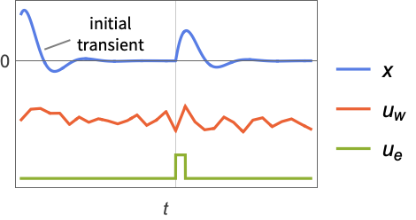
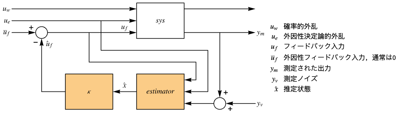
- 調整コントローラは系を乱そうとする外乱 uwおよび ueがあっても系を平衡状態に保とうとする.典型的な例として,直立した倒立振子や水平飛行中の航空機等が挙げられる.
- 調整コントローラは
 の形の制御規則で与えられる.ただし,
 は計算されたゲイン行列である.
- 状態 x の重み q,r,p およびフィードバック入力 ufの二次費用関数は以下で与えられる.
-

連続時間系 
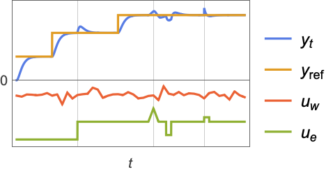
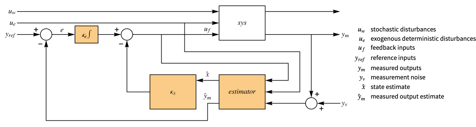
離散時間系 - 追跡コントローラは,それを妨害する外乱 uwおよび ueがあっても参照信号を追跡しようとする.典型的な例として,自動車のクルーズコントロールシステムやロボットの経路追跡が挙げられる.
- 追跡コントローラは
 の形の制御規則で与えられる.ただし,
 は系 sys と
 のダイナミクスを含む拡張系のための計算されたゲイン行列である.
- 拡張状態
 の重み q,r ,p およびフィードバック入力 ufの二次費用関数は以下で与えられる.
-

連続時間系 
離散時間系 - 拡張系の状態の数は
 で与えられる.ただし,
 は sys のSystemsModelOrderで,
 は yrefの次数で,
 は信号 yrefの数で与えられる.
- 重み行列の選択は,結果としてパフォーマンスと制御努力のトレードオフとなり,優れた設計に反復的に到達する.初期値は成分が
 の対角行列でよい.ただし,ziは対応する xiまたは uiの許容可能な最大絶対値である.
- 重み wts は次の形でよい.
-
{q,r} クロスカップリングがない費用関数 {q,r,p} クロスカップリング行列 p がある費用関数 - 測定値 ymは
 としてモデル化できる.ただし,
 および
 は
 に関連付けられた
 および
 の部分行列で,
 はノイズである.
- 確率的入力 uwおよび測定ノイズ yvは,ゼロ平均,ガウス,ホワイトのノイズであるとみなされる.
-
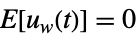 ,

過程ノイズ 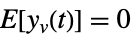 ,

測定ノイズ 
相互共分散 - 共分散行列 cvs は以下の形でよい.
-
{w,v} 共分散行列とゼロ相互共分散 {w,v,h} 共分散行列と相互共分散行列 - 系の指定 sspec は,系 sys と uf,ue,yt,yrefの指定である.
- 系の指定 sspec は以下の形でよい.
-
StateSpaceModel[…] 線形制御入力と線形状態 AffineStateSpaceModel[…] 線形制御入力と非線形状態 NonlinearStateSpaceModel[…] 非線形制御入力と非線形状態 SystemModel[…] 一般的な系のモデル <…> Associationとして与えられる詳細な系の指定 - 系の指定の詳細は次のキーを持つことができる.
-
"InputModel" sys モデルの任意のもの "FeedbackInputs" All フィードバック入力 uf "ExogenousInputs" None 外因的な入力 ue "MeasuredOutputs" All 測定された出力 ym "TrackedOutputs" None 追跡された出力 yt "TrackedSignal" Automatic yrefのダイナミクス - 入力と出力は以下の形でよい.
-
{num1,…,numn} StateSpaceModel,AffineStateSpaceModel,NonlinearStateSpaceModelで使われる番号付きの入力または出力 numi {name1,…,namen} SystemModelで使われる名前付きの入力または出力 namei All すべての入力または出力を使う None 入力または出力は使わない - LQGRegulator[…,"Data"]は,cd["prop"]の形で追加的な特性の抽出に使えるSystemsModelControllerDataオブジェクト cd を返す.
- LQGRegulator[…,"prop"]を使って cd["prop"]の値を直接得ることができる.
- 次は,特性"prop"の可能な値である.
-
"BlockDiagram" csys のブロック図 {"BlockDiagram","SampledData"True} csys のサンプルデータブロック図を作成する "ClosedLoopPoles" "ClosedLoopSystem"の極 "ClosedLoopSystem" 系 csys {"ClosedLoopSystem",cspec} 閉ループ系の形に対する詳細な制御 "ControllerModel" モデル cm "Design" コントローラ設計のタイプ "EstimatorGains" ゲイン行列 ℓ "EstimatorGainsDesignModel" 推定器ゲインの設計に使われるモデル "EstimatorRegulatorFeedbackModel" ue, ymを入力として,  を出力として持つモデル
"EstimatorRegulatorModel" uf, ue, ymを入力として,  を出力として持つモデル erm
"ExogenousInputs" 決定論的入力 ueと非フィードバック入力 sys "FeedbackGains" ゲイン行列 κ またはそれに相当するもの "FeedbackGainsDesignModel" フィードバックゲインの設計に使われモデル "FeedbackGainsModel" モデル gm または{gm1,gm2} "FeedbackInputs" フィードバックに使われる sys の入力 uf "InputCount" sys の入力数 u "InputModel" 入力モデル sys "MeasuredOutputs" sys の測定された出力 ym "OpenLoopPoles" テイラー(Taylor )線形化 sys の極 "OutputCount" sys の出力の数 y "SamplingPeriod" sys のサンプリング周期 "StateCount" sys の x の状態数 "StateEstimatorModel" モデル sem "StateOutputEstimatorModel" モデル soem "TrackedOutputs" 追跡された sys の出力 yt - 次は,cspec の可能なキーである.
-
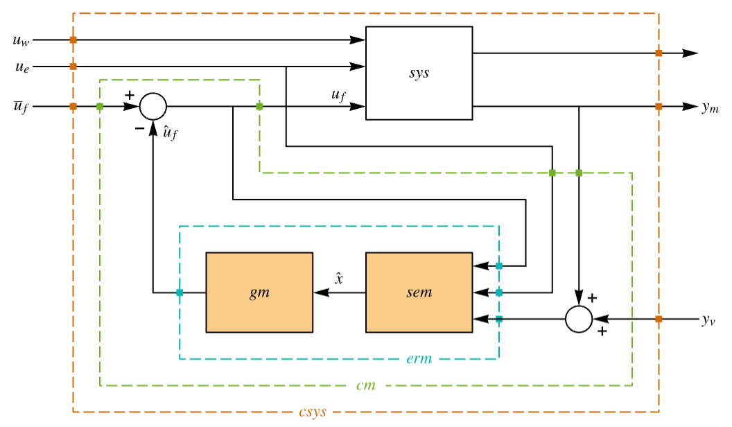
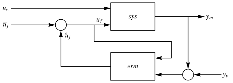
"InputModel" csys の入力モデル "Merge" csys をマージするかどうか "ModelName" csys の名前 "SamplingPeriod" サンプルデータ csys を作成する - 次は,調整器のレイアウトの線図である.
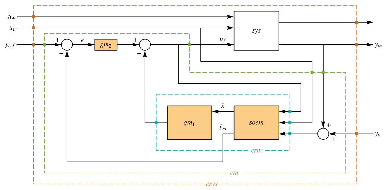
- 次は,追跡器のレイアウトの線図である.
例題
すべて開く すべて閉じる例 (4)
フィードバック入力が uf でプロセスノイズ入力が uw である系の指定 sspec:
sspec = <|"InputModel" -> StateSpaceModel[{{{0, 1}, {-3, -0.5}}, {{0, 1}, {1, 0}}, {{1, 0}}, {{0, 0}}},
SamplingPeriod -> None, SystemsModelLabels -> {{uf, uw}}], "FeedbackInputs" -> 1|>;cvs = {(10^2), (10)};wts = {(| | |
| ---- | ---- |
| 10^4 | 0 |
| 0 | 10^2 |), (10^2)};LQGRegulator[sspec, cvs, wts]nsys = NonlinearStateSpaceModel[{{-1 + 2*Subscript[x, 2],
u + 4*Subscript[x, 1] - Subscript[x, 2]},
{Subscript[x, 1] + 3*Subscript[x, 2]}},
{{Subscript[x, 1], 1}, {Subscript[x, 2], 1}}, {{u, 1}},
{Automatic}, Automatic, SamplingPeriod -> None];cvs = {{{}}, (10^-3)};wts = {(| | |
| - | -- |
| 1 | 0 |
| 0 | 10 |), {{1}}};LQGRegulator[nsys, cvs, wts]//Nフィードバック入力 uf,プロセスノイズ入力 uw ,追跡された出力 ym の系:
sspec = <|"InputModel" -> StateSpaceModel[{{{0, 1}, {-2, -1.5}}, {{0, 2}, {1, 0}}, {{1, 0}}, {{0, 0}}},
 SamplingPeriod -> None, SystemsModelLabels -> {{uf, uw},
{ym}}], "TrackedOutputs" -> 1, "FeedbackInputs" -> 1|>;cvs = {(10^2), (10)};wts = {(| | | |
| ---- | ---- | ---- |
| 10^4 | 0 | 0 |
| 0 | 10^2 | 0 |
| 0 | 0 | 10^2 |), (10^2)};LQGRegulator[sspec, cvs, wts]//Nsspec = <|"InputModel" -> StateSpaceModel[{{{0, 1, 4}, {-6, 5, 1}, {0, 0, 2}}, {{0, 1}, {2, 0}, {1, 0}},
{{0.4, 0.2, 0}, {0, 1, 0}}, {{0., 0}, {0, 0}}}, SamplingPeriod -> None,
SystemsModelLabels -> {{uf, uw}}], "FeedbackInputs" -> 1|>;cvs = {{{10^2}}, (| | |
| - | - |
| 1 | 0 |
| 0 | 1 |)};wts = {(| | | |
| - | - | - |
| 2 | 0 | 0 |
| 0 | 2 | 0 |
| 0 | 0 | 5 |), (1)};lqgr = LQGRegulator[sspec, cvs, wts, "Data"]安定した閉ループ系と不安定な開ループ系の極は s 平面の左半平面と右半平面にある:
PoleZeroPlot[{lqgr["InputModel"], lqgr["ClosedLoopSystem"]//Chop}, PlotLegends -> {"ol pole", "ol zero", "cl pole", "cl zero"}]スコープ (34)
基本的な用法 (4)
1つのフィードバック入力 uf と1つのノイズのある測定値 ym を持つ系:
ssm  = StateSpaceModel[{{{2, 1}, {-1.5, -2}}, {{-1}, {1}}, {{1, 0}}, {{0}}}, SamplingPeriod -> None,
 SystemsModelLabels -> {uf, ym}];
ノイズのある入力がないので,入力の共分散行列 cvs は空である:
cvs = {{{}}, (1)};wts = {(| | |
| - | - |
| 1 | 0 |
| 0 | 1 |), (2)};LQRegulatorGains[ssm, {{{0, 0}, {0, 0}}, {{1}}, {{0}, {0}}}]sspec = <|"InputModel" -> ssm, "FeedbackInputs" -> 1, "MeasuredOutputs" -> 1|>;
LQGRegulator[sspec, cvs, wts]1つのフィードバック入力 uf,1つのノイズのある入力 uw,1つのノイズのある測定値 ym がある系:
sspec = <|"InputModel" -> StateSpaceModel[{{{0, -1.5}, {1., -2.}}, {{1, 0.1}, {0, 0}}, {{0, 1.}}, {{0, 0}}},
 SamplingPeriod -> None, SystemsModelLabels -> {{uf, uw},
ym, None}], "FeedbackInputs" -> 1, "MeasuredOutputs" -> 1|>;{cvs, wts} = {{(1), (1)}, {(| | |
| - | - |
| 1 | 0 |
| 0 | 1 |), (2)}};LQGRegulator[sspec, cvs, wts]sspec = <|"InputModel" -> StateSpaceModel[{{{0, -1.5}, {1., -2.}}, {{1, 0.1, 0}, {0, 0, 0.5}}, {{0, 1.}}, {{0, 0, 0}}},
SamplingPeriod -> None, SystemsModelLabels ->
{{uf, uw, ue}, ym, None}], "FeedbackInputs" -> 1, "ExogenousInputs" -> 3, "MeasuredOutputs" -> 1|>;{cvs, wts} = {{(1), (1)}, {(| | |
| - | - |
| 1 | 0 |
| 0 | 1 |), (2)}};LQGRegulator[sspec, cvs, wts]sspec = <|"InputModel" -> StateSpaceModel[{{{0, -2, 0, 0}, {1, -3, 0, 0}, {0, 0, 0, -2}, {0, 0, 1, -3}},
{{0, 1, -2}, {1, 1, -1}, {3, 2, 2}, {0, 1, 1}}, {{0, 1, 0, 0}, {0, 0, 0, 1}},
{{0, 0, 1}, {0, 0, 0}}}, SamplingPeriod -> None, SystemsModelLabels ->
{{uf1, uw, uf2}, {ym1, ym2},
None}], "FeedbackInputs" -> {1, 3}, "MeasuredOutputs" -> {1, 2}|>;{cvs, wts} = {{(0.5), (| | |
| ---- | ---- |
| 0.25 | 0 |
| 0 | 0.25 |)}, {(| | | | |
| -- | -- | -- | -- |
| 10 | 0 | 0 | 0 |
| 0 | 10 | 0 | 0 |
| 0 | 0 | 10 | 0 |
| 0 | 0 | 0 | 10 |), (| | |
| - | - |
| 1 | 0 |
| 0 | 1 |)}};LQGRegulator[sspec, cvs, wts]//N工場モデル (7)
連続時間StateSpaceModel:
LQGRegulator[StateSpaceModel[{{{1, 1.}, {-1, -3.5}}, {{0}, {1}}, {{1, 0}}, {{0}}}, SamplingPeriod -> None,
SystemsModelLabels -> None], {{{}}, (0.5)}, {(| | |
| - | - |
| 1 | 0 |
| 0 | 1 |), (1)}]離散時間StateSpaceModel:
LQGRegulator[StateSpaceModel[{{{1, 1.}, {-1, -3.5}}, {{0}, {1}}, {{1, 0}}, {{0}}},
SamplingPeriod -> τ, SystemsModelLabels -> None], {{{}}, (0.5)}, {(| | |
| - | - |
| 1 | 0 |
| 0 | 1 |), (1)}]ディスクリプタStateSpaceModel:
LQGRegulator[StateSpaceModel[{{{-2, -1}, {0, 1}}, {{1}, {0}}, {{1, 0}}, {{1}}, {{1, 0}, {1, 1}}},
{{x1[t], 0}, {x2[t], 0}},
{{u[t], 0}}, Automatic, t, SamplingPeriod -> None,
SystemsModelLabels -> None], {{{}}, (0.5)}, {(| | |
| - | - |
| 1 | 0 |
| 0 | 1 |), (1.0)}]LQGRegulator[AffineStateSpaceModel[{{Sin[Subscript[x, 1]] + Subscript[x, 2],
-Subscript[x, 1] - 2*Subscript[x, 2]},
{{Subscript[x, 1]}, {1}}, {Subscript[x, 1]}, {{0}}},
{Subscript[x, 1], Subscript[x, 2]}, {{u, 0}},
{y}, Automatic, SamplingPeriod -> None], {{{}}, (2.0)}, {(| | |
| - | - |
| 1 | 0 |
| 0 | 1 |), (1.0)}]LQGRegulator[NonlinearStateSpaceModel[
{{Subscript[x, 2] + Subscript[x, 1]*Subscript[x, 2],
u + Subscript[x, 1]}, {Subscript[x, 1]}},
{Subscript[x, 1], Subscript[x, 2]}, {u}, {y},
Automatic, SamplingPeriod -> None], {{{}}, (0.5)}, {(| | |
| - | - |
| 1 | 0 |
| 0 | 1 |), (1.0)}]sm = CreateSystemModel[{x1'[t] == -2 x1[t] + x2[t] + u[t], x2'[t] == 2 x1[t] + x2[t] + u[t], y[t] == x1[t]}, t, {"u"∈"Modelica.Blocks.Interfaces.RealInput", "y"∈"Modelica.Blocks.Interfaces.RealOutput"}];LQGRegulator[sm, {{{}}, (2)}, {(| | |
| - | - |
| 1 | 0 |
| 0 | 1 |), (1.0)}]ノイズのある入力があるSystemModel:
sm = CreateSystemModel[{x1'[t] == -x1[t] + x2[t] + uf[t], x2'[t] == x1[t] + x2[t] + uf[t] + ue[t], y[t] == x1[t]}, t, {{"uf", "ue"}∈"Modelica.Blocks.Interfaces.RealInput", "y"∈"Modelica.Blocks.Interfaces.RealOutput"}];sspec = <|"InputModel" -> sm, "FeedbackInputs" -> "uf"|>;LQGRegulator[sspec, {(1), (2)}, {(| | |
| - | - |
| 1 | 0 |
| 0 | 1 |), (1.0)}]特性 (15)
デフォルトで,LQGRegulatorは推定器と調整器を含むコントローラを返す:
sspec = <|"InputModel" -> StateSpaceModel[{{{0, -6}, {1, -5}}, {{1, -6}, {1, -3}}, {{0, 1}}, {{0, 1}}},
SamplingPeriod -> None, SystemsModelLabels -> None], "FeedbackInputs" -> 1|>;
{cvs, wts} = {{(1), (0.5)}, {(| | |
| - | - |
| 1 | 0 |
| 0 | 1 |), (1.0)}};LQGRegulatorを組み立てる:
LQGRegulator[sspec, cvs, wts]LQGRegulatorモデル:
LQGRegulator[sspec, cvs, wts, "EstimatorRegulatorModel"]sspec = <|"InputModel" -> StateSpaceModel[{{{0, -6}, {1, -5}}, {{1, -6}, {1, -3}}, {{0, 1}}, {{0, 1}}},
SamplingPeriod -> None, SystemsModelLabels -> None], "FeedbackInputs" -> 1|>;
{cvs, wts} = {{(1), (0.5)}, {(| | |
| - | - |
| 1 | 0 |
| 0 | 1 |), (1.0)}};LQGRegulator[sspec, cvs, wts, "FeedbackGains"]sspec = <|"InputModel" -> StateSpaceModel[{{{0, -6}, {1, -5}}, {{1, -6}, {1, -3}}, {{0, 1}}, {{0, 1}}},
SamplingPeriod -> None, SystemsModelLabels -> None], "FeedbackInputs" -> 1|>;
{cvs, wts} = {{(1), (0.5)}, {(| | |
| - | - |
| 1 | 0 |
| 0 | 1 |), (1.0)}};LQGRegulator[sspec, cvs, wts, "FeedbackGainsModel"]sspec = <|"InputModel" -> StateSpaceModel[{{{0, -6}, {1, -5}}, {{1, -6}, {1, -3}}, {{0, 1}}, {{0, 1}}},
SamplingPeriod -> None, SystemsModelLabels -> None], "FeedbackInputs" -> 1|>;
{cvs, wts} = {{(1), (0.5)}, {(| | |
| - | - |
| 1 | 0 |
| 0 | 1 |), (1.0)}};LQGRegulator[sspec, cvs, wts, "FeedbackGainsDesignModel"]sspec = <|"InputModel" -> StateSpaceModel[{{{0, -6}, {1, -5}}, {{1, -6}, {1, -3}}, {{0, 1}}, {{0, 1}}},
SamplingPeriod -> None, SystemsModelLabels -> None], "FeedbackInputs" -> 1|>;
{cvs, wts} = {{(1), (0.5)}, {(| | |
| - | - |
| 1 | 0 |
| 0 | 1 |), (1.0)}};LQGRegulator[sspec, cvs, wts, "EstimatorGains"]sspec = <|"InputModel" -> StateSpaceModel[{{{0, -6}, {1, -5}}, {{1, -6}, {1, -3}}, {{0, 1}}, {{0, 1}}},
SamplingPeriod -> None, SystemsModelLabels -> None], "FeedbackInputs" -> 1|>;
{cvs, wts} = {{(1), (0.5)}, {(| | |
| - | - |
| 1 | 0 |
| 0 | 1 |), (1.0)}};LQGRegulator[sspec, cvs, wts, "StateEstimatorModel"]sspec = <|"InputModel" -> StateSpaceModel[{{{0, -6}, {1, -5}}, {{1, -6}, {1, -3}}, {{0, 1}}, {{0, 1}}},
SamplingPeriod -> None, SystemsModelLabels -> None], "FeedbackInputs" -> 1|>;
{cvs, wts} = {{(1), (0.5)}, {(| | |
| - | - |
| 1 | 0 |
| 0 | 1 |), (1.0)}};LQGRegulator[sspec, cvs, wts, "EstimatorGainsDesignModel"]非線形系については,推定器の設計に使われるモデルは非線形状態空間モデルである:
sspec = <|"InputModel" -> AffineStateSpaceModel[{{-7*Subscript[x, 2] + Subscript[x, 2]/
E^Subscript[x, 1], Subscript[x, 1] -
5*Subscript[x, 2]}, {{1, -6}, {1 + Subscript[x, 1], -3}},
{Subscript[x, 2]}, {{0, 1}}}, {Subscript[x, 1],
Subscript[x, 2]}, {Subscript[u, 1], Subscript[u, 2]},
{y}, Automatic, SamplingPeriod -> None], "FeedbackInputs" -> 1|>;
{cvs, wts} = {{(1), (0.5)}, {(| | |
| - | - |
| 1 | 0 |
| 0 | 1 |), (1.0)}};LQGRegulator[sspec, cvs, wts, "EstimatorGainsDesignModel"]LQGRegulator[sspec, cvs, wts, "FeedbackGainsDesignModel"]StateSpaceModel[sspec["InputModel"]]コントローラは直列化された推定器ゲインとフィードバックゲインである:
sspec = <|"InputModel" -> StateSpaceModel[{{{0, -6}, {1, -5}}, {{1, -6}, {1, -3}}, {{0, 1}}, {{0, 1}}},
SamplingPeriod -> None, SystemsModelLabels -> None], "FeedbackInputs" -> 1|>;
{cvs, wts} = {{(1), (0.5)}, {(| | |
| - | - |
| 1 | 0 |
| 0 | 1 |), (1.0)}};SystemsModelSeriesConnect@@LQGRegulator[sspec, cvs, wts, { "StateEstimatorModel", "FeedbackGainsModel"}]LQGRegulator[sspec, cvs, wts]sspec = <|"InputModel" -> StateSpaceModel[{{{0, -6}, {1, -5}}, {{1, -6}, {1, -3}}, {{0, 1}}, {{0, 1}}},
SamplingPeriod -> None, SystemsModelLabels -> None], "FeedbackInputs" -> 1|>;
{cvs, wts} = {{(1), (0.5)}, {(| | |
| - | - |
| 1 | 0 |
| 0 | 1 |), (1.0)}};LQGRegulator[sspec, cvs, wts, "ClosedLoopSystem"]sspec = <|"InputModel" -> StateSpaceModel[{{{0, -6}, {1, -5}}, {{1, -6}, {1, -3}}, {{0, 1}}, {{0, 1}}},
SamplingPeriod -> None, SystemsModelLabels -> None], "FeedbackInputs" -> 1|>;
{cvs, wts} = {{(1), (0.5)}, {(| | |
| - | - |
| 1 | 0 |
| 0 | 1 |), (1.0)}};LQGRegulator[sspec, cvs, wts, "BlockDiagram"]sspec = <|"InputModel" -> StateSpaceModel[{{{0, -6}, {1, -5}}, {{1, -6}, {1, -3}}, {{0, 1}}, {{0, 1}}},
SamplingPeriod -> None, SystemsModelLabels -> None], "FeedbackInputs" -> 1|>;
{cvs, wts} = {{(1), (0.5)}, {(| | |
| -- | -- |
| 10 | 0 |
| 0 | 10 |), (1.0)}};LQGRegulator[sspec, cvs, wts, "ClosedLoopPoles"]LQGRegulator[IconizedObject[«sspec»], IconizedObject[«cvs»], IconizedObject[«wts»], "Design"]Dataset[Table[{prop, LQGRegulator[IconizedObject[«sspec»], IconizedObject[«cvs»], IconizedObject[«wts»], prop]}, {prop, IconizedObject[«props»]}]]lqr = LQGRegulator[IconizedObject[«sspec»], IconizedObject[«cvs»], IconizedObject[«wts»], "Data"]lqr["Properties"]lqr["EstimatorGains"]追跡 (5)
sspec = <|"InputModel" -> StateSpaceModel[{{{0, 1}, {-5, -3}}, {{0}, {1}}, {{5, 0}}, {{0}}}, SamplingPeriod -> None,
SystemsModelLabels -> None], "TrackedOutputs" -> 1|>;
𝒸𝒹 = LQGRegulator[sspec, {{{}}, (1)}, {(| | | |
| -- | --- | -- |
| 10 | 0 | 0 |
| 0 | 0.5 | 0 |
| 0 | 0 | 10 |), {{0.1}}}, "Data"]
OutputResponse[Chop[𝒸𝒹["ClosedLoopSystem"]], {1, 0}, {t, 0, 3}];
Plot[{1, %}, {t, 0, 3}, IconizedObject[«plotOpts»]]𝒸𝒹["BlockDiagram"]sspec = <|"InputModel" -> StateSpaceModel[{{{0, 1.}, {0.5, -2.3}}, {{0}, {1.}}, {{1., 0}}, {{0}}}, SamplingPeriod -> 0.05,
SystemsModelLabels -> None], "TrackedOutputs" -> 1|>;𝒸𝒹 = LQGRegulator[sspec, {{{}}, (1)}, {(| | | |
| - | -- | --- |
| 1 | 0 | 0 |
| 0 | 10 | 0 |
| 0 | 0 | 100 |), {{0.1}}}, "Data"]
ref = {Table[1, 15]};
or = OutputResponse[𝒸𝒹["ClosedLoopSystem"], ref];ListLinePlot[Join[ref, or], IconizedObject[«plotOpts»]]sspec = <|"InputModel" -> StateSpaceModel[{{{0, 1}, {-3, -0.5}}, {{0, 1}, {1, -1}}, {{1, 0}, {1, 1}}, {{0, 0}, {0, 0}}},
SamplingPeriod -> None, SystemsModelLabels -> None], "TrackedOutputs" -> {1, 2}|>;𝒸𝒹 = LQGRegulator[sspec, {{{}}, {{0.1, 0}, {0, 0.1}}}, DiagonalMatrix /@ {{1, 1, 5, 10}, {1, 1}}, "Data"]𝒸𝒹["ClosedLoopSystem"]refs = RandomInteger[{-20, -4}, 2];
or = OutputResponse[𝒸𝒹["ClosedLoopSystem"], Join[refs, {0, 0}], {t, 0, 15}];Plot[Evaluate[Riffle[refs, or]], {t, 0, 15}, IconizedObject[«plotOpts»]]sspec = <|"InputModel" -> StateSpaceModel[{{{0, 1}, {-5, -3}}, {{0}, {1}}, {{5, 0}}, {{0}}}, SamplingPeriod -> None,
SystemsModelLabels -> None], "TrackedOutputs" -> 1|>;𝒸𝒹 = LQGRegulator[sspec, {{{}}, (1)}, {(| | | |
| - | --- | ---- |
| 1 | 0 | 0 |
| 0 | 100 | 0 |
| 0 | 0 | 10^3 |), {{1}}}, "Data"]cm = 𝒸𝒹["ControllerModel"]//N//Chopref = {1};
csys = 𝒸𝒹["ClosedLoopSystem"];
n = SystemsModelOrder[sspec["InputModel"]];cinps = Join[ref, OutputResponse[csys, ref, {t, 0, 5}], StateResponse[csys, ref, {t, 0, 5}][[1 ;; n]]]OutputResponse[cm, cinps, {t, 0, 5}];
Plot[%, {t, 0, 5}, PlotRange -> All]tSig = Function[{r, t}, 9.016 r[t] + 0.8003 Derivative[1][r][t] + 10.0096 Derivative[2][r][t] + 0.16 Derivative[3][r][t] + Derivative[4][r][t]]m = Max[Join[Cases[tSig[r, t], Derivative[n_][r][t] :> n, Infinity], {0}]]ics = {r[0] == 0, r'[0] == 0, r''[0] == 0, r'''[0] == 1};ref = r[t] /. DSolve[Join[{tSig[r, t] == 0}, ics], r[t], t];Plot[ref, {t, 0, 30}, PlotRange -> All]sspec = <|"InputModel" -> StateSpaceModel[{{{-1}}, {{1}}, {{1}}, {{0}}}, SamplingPeriod -> None, SystemsModelLabels -> None], "TrackedOutputs" -> {1}, "TrackedSignal" -> tSig|>;{q, k} = {Length[sspec["TrackedOutputs"]], SystemsModelOrder[sspec["InputModel"]]}{qq, rr} = {DiagonalMatrix[{1, 100, 10, 10, 10}], {{0.1}}};
Join[Dimensions[qq], {k + m q}]𝒸𝒹 = LQGRegulator[sspec, {{{}}, {{1}}}, {qq, rr}, "Data"]OutputResponse[𝒸𝒹["ClosedLoopSystem"], ref, {t, 0, 30}];
Plot[{ref, %[[1]]}, {t, 0, 30}, IconizedObject[«plotOpts»]]閉ループ系 (3)
1つの外乱入力がある非線形工場モデルのための閉ループ系を組み立てる:
sspec = <|"InputModel" -> AffineStateSpaceModel[{{-Subscript[x, 2] + Subscript[x, 1]*
     Subscript[x, 2], Subscript[x, 1] + Subscript[x, 1]^2 -
    Subscript[x, 1]*Subscript[x, 2]},
  {{0, 1}, {1 + Subscript[x, 1], 0}}, {Subscript[x, 1]}, {{0, 0}}},
 {Subscript[x, 1], Subscript[x, 2]},
 {Subscript[u, 1], Subscript[u, 2]}, {Automatic}, Automatic,
SamplingPeriod -> None], "FeedbackInputs" -> 1|>;cvs = {(10^2), (10.0)};
wts = {(| | |
| ---- | ---- |
| 10^4 | 0.0 |
| 0.0 | 10^2 |), (10^2)};csys1 = LQGRegulator[sspec, cvs, wts, "ClosedLoopSystem"]//Chopsspeclin = <|"InputModel" -> StateSpaceModel[AffineStateSpaceModel[{{-Subscript[x, 2] + Subscript[x, 1]*
Subscript[x, 2], Subscript[x, 1] + Subscript[x, 1]^2 -
Subscript[x, 1]*Subscript[x, 2]},
{{0, 1}, {1 + Subscript[x, 1], 0}}, {Subscript[x, 1]}, {{0, 0}}},
{Subscript[x, 1], Subscript[x, 2]},
{Subscript[u, 1], Subscript[u, 2]}, {Automatic}, Automatic,
SamplingPeriod -> None]], "FeedbackInputs" -> 1|>csys2 = LQGRegulator[sspeclin, cvs, wts, "ClosedLoopSystem"]//ChopTable[OutputResponse[{sys, {0.1, -1, 0, 0}}, {0, 0}, {t, 0, 20}], {sys, {csys1, csys2}}];
Plot[%, {t, 0, 20}, IconizedObject[«plotOpts»]]LQGRegulatorで工場のマージされた閉ループ系を組み立てる:
sspec = <|"InputModel" -> StateSpaceModel[{{{-0.3, 0.2}, {0.15, -0.25}}, {{2, 10}, {7, -2}}, {{1, -4}}, {{0, 0}}},
SamplingPeriod -> 1, SystemsModelLabels -> None], "FeedbackInputs" -> 1|>;{cvs, wts} = {{(0.0001), (1)}, {(| | |
| ----- | ----- |
| 0.001 | 0 |
| 0 | 0.001 |), (0.1)}};LQGRegulator[sspec, cvs, wts, "ClosedLoopSystem"]umlqg = LQGRegulator[sspec, cvs, wts, {"ClosedLoopSystem", <|"Merge" -> False|>}]SystemsModelMerge[umlqg]LQGRegulator[sspec, cvs, wts, {"ClosedLoopSystem", <|"Merge" -> True|>}]sm = CreateSystemModel["LiquidLevelSystem", {r c h'[t] + h[t] == r (qi[t] + qd[t]), y[t] == h[t]}, t, {{"qi", "qd"}∈"Modelica.Blocks.Interfaces.RealInput", "y"∈"Modelica.Blocks.Interfaces.RealOutput"}, <|"ParameterValues" -> {r -> 0.01, c -> 10}|>];csysName = "LiquidLevelControlSystem";
csys = LQGRegulator[<|"InputModel" -> sm, "FeedbackInputs" -> "qd"|>, {{{0.1}}, {{0.001}}}, {{{1}}, {{5}}}, {"ClosedLoopSystem", <|"ModelName" -> csysName|>}]csys["ModelName"]SystemModel[csysName] /@ {"InputVariables", "OutputVariables"}アプリケーション (11)
機械系 (3)
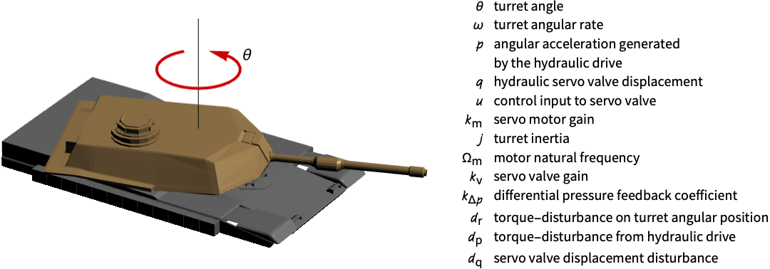
turret = StateSpaceModel[IconizedObject[«eqns»] /. IconizedObject[«pars»], {θ[t], ω[t], 𝓅[t], 𝓆[t]},
	{𝓊[t], Subscript[𝒹, r][t], Subscript[𝒹, p][t], Subscript[𝒹, q][t]}, {θ[t], 𝓆[t]}, t, IconizedObject[«labels»]]
砲塔の向きは,次の状態での初期外乱に対しては調整されていない:
OutputResponse[{turret, {0.6, 0, 0, 0.5}}, {0, 0, 0, 0}, {t, 0, 0.1}];
Plot[%, {t, 0, 0.1}, PlotRange -> All, PlotLegends -> {θ, 𝓆}]sspec = <|"InputModel" -> turret, "FeedbackInputs" -> 1|>;cvs = {10^-1DiagonalMatrix[{1, 1, 1}], 10^-4DiagonalMatrix[{1, 1}]};
wts = {DiagonalMatrix[{200, 1, 1, 1}], {{0.1}}};lqg = LQGRegulator[sspec, cvs, wts, "Data"]csys = lqg[{"ClosedLoopSystem", <|"Merge" -> True|>}]ノイズが多い信号を生成して過程ノイズのシミュレーションを行う:
n = 100;
Thread[{Range[0, n], RandomVariate[NormalDistribution[0, Sqrt[3 10^-3]], {n + 1}]}];
Plot[Subscript[u, w] = Interpolation[%, t], {t, 0, n}]Thread[{Range[0, n], RandomVariate[NormalDistribution[0, Sqrt[ 10^-3]], {n + 1}]}];
Plot[Subscript[y, v] = Interpolation[%, t], {t, 0, n}]or = OutputResponse[{csys, {0.6, 0, 0, 0.5}}, {0, 0, 0, 0, Subscript[u, w], Subscript[y, v]}, {t, 0, 10}];
Plot[%, {t, 0, 10}, PlotRange -> All, PlotLegends -> {θ, 𝓆}]cm = lqg["ControllerModel"]OutputResponse[cm, Join[{0}, or], {t, 0, 10}];
Plot[%, {t, 0, 10}, PlotRange -> All]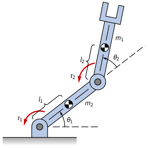
Simplify[NonlinearStateSpaceModel[IconizedObject[«eqns»], IconizedObject[«eqAngles»], IconizedObject[«eqTorques»], {Subscript[θ, 1][t], Subscript[θ, 2][t]}, t] /. IconizedObject[«pars»]];
robot = NonlinearStateSpaceModel[%, Automatic, Automatic, Automatic, None]OutputResponse[robot, {0, 0}, {t, 0, 10}];
Plot[%, {t, 0, 10}, PlotLegends -> {Subscript[θ, 1], Subscript[θ, 2]}]cvs = {{{}}, DiagonalMatrix[{10^2, 10^2}]};
wts = {DiagonalMatrix[{200, 1, 100, 1}], DiagonalMatrix[{(1/48^2), (1/48^2)}]};lqg = LQGRegulator[robot, cvs, wts, "Data"]Style[csys = lqg["ClosedLoopSystem"]//FullSimplify, Small]ノイズがある信号を生成してセンサーノイズのシミュレーションを行う:
n = 100;Thread[{Range[0, n], RandomVariate[NormalDistribution[0, Sqrt[3 10^-3]], {n + 1}]}];
Plot[Subscript[y, v] = Interpolation[%, t], {t, 0, n}]sr = StateResponse[{csys, {0.1, 0, 0.2, 0}}, {0, 0, 0, Subscript[y, v]}, {t, 0, 10}];
Plot[{%[[1]], %[[3]]}, {t, 0, 10}, PlotRange -> All, PlotLegends -> {Subscript[θ, 1], Subscript[θ, 2]}]Style[cm = lqg["ControllerModel"]//FullSimplify, Small]OutputResponse[cm, Join[{0, 0}, {sr[[1]], sr[[3]]}], {t, 0, 5}];
Plot[%, {t, 0, 5}, PlotRange -> All, PlotLegends -> {Subscript[𝒯, 1], Subscript[𝒯, 2]}]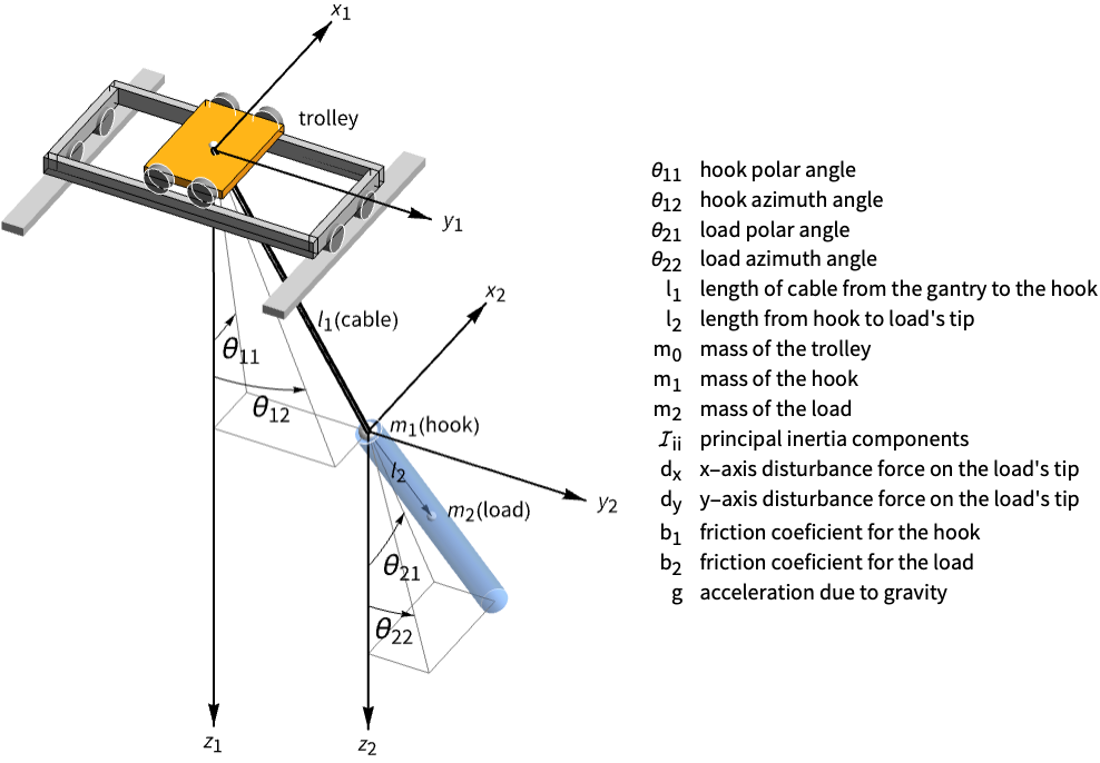
crane = StateSpaceModel[IconizedObject[«eqns»] /. IconizedObject[«pars»], IconizedObject[«vars»], IconizedObject[«inps»], IconizedObject[«outs»], t, IconizedObject[«labels»]]OutputResponse[crane, {0, 0, 100UnitBox[(t/3) - 1], 80UnitBox[(t/3) - 1]}, {t, 0, 20}];
Table[Plot[ℴ𝓇[[1]], {t, 0, 15}, IconizedObject[«plotOpts»]], {ℴ𝓇, ({%, {Subscript[θ, 11], Subscript[θ, 12], Subscript[θ, 21], Subscript[θ, 22]}})}]sspec = <|"InputModel" -> crane, "FeedbackInputs" -> {1, 2}|>;cvs = {(| | |
| ---- | ---- |
| 1000 | 0 |
| 0 | 1000 |), (| | | | |
| -------- | -------- | -------- | -------- |
| (1/1000) | 0 | 0 | 0 |
| 0 | (1/1000) | 0 | 0 |
| 0 | 0 | (1/1000) | 0 |
| 0 | 0 | 0 | (1/1000) |)};q = (| | | | | | | | |
| ----------- | ------------ | ----------- | ------------ | ----------- | ------------ | ----------- | ------------ |
| (1/maxθ112) | 0 | 0 | 0 | 0 | 0 | 0 | 0 |
| 0 | (1/maxθp112) | 0 | 0 | 0 | 0 | 0 | 0 |
| 0 | 0 | (1/maxθ122) | 0 | 0 | 0 | 0 | 0 |
| 0 | 0 | 0 | (1/maxθp122) | 0 | 0 | 0 | 0 |
| 0 | 0 | 0 | 0 | (1/maxθ212) | 0 | 0 | 0 |
| 0 | 0 | 0 | 0 | 0 | (1/maxθp212) | 0 | 0 |
| 0 | 0 | 0 | 0 | 0 | 0 | (1/maxθ222) | 0 |
| 0 | 0 | 0 | 0 | 0 | 0 | 0 | (1/maxθp222) |) /. IconizedObject[«qspec»];r = (| | |
| ---------- | ---------- |
| (1/maxx02) | 0 |
| 0 | (1/maxy02) |) /. IconizedObject[«rspec»];lqg = LQGRegulator[sspec, cvs, {q, r}, "Data"]csys = lqg[{"ClosedLoopSystem", <|"Merge" -> True|>}]//Chopノイズのある信号を生成して過程のノイズのシミュレーションを行う:
n = 100;Thread[{Range[0, n], RandomVariate[NormalDistribution[0, Sqrt[0.15]], {n + 1}]}];
Plot[Subscript[u, w] = Interpolation[%, t], {t, 0, n}]Thread[{Range[0, n], RandomVariate[NormalDistribution[0, Sqrt[0.075]], {n + 1}]}];
Plot[Subscript[y, v] = Interpolation[%, t], {t, 0, n}]or = OutputResponse[csys, {Subscript[u, w], Subscript[y, v], 10^2UnitBox[(t/3) - 1] + Subscript[u, w], 80UnitBox[(t/3) - 1] + Subscript[u, w]}, {t, 0, 60}];
Table[Plot[ℴ𝓇[[1]], {t, 0, 15}, IconizedObject[«plotOpts»]], {ℴ𝓇, ({%, {Subscript[θ, 11], Subscript[θ, 12], Subscript[θ, 21], Subscript[θ, 22]}})}]cm = lqg[{"ControllerModel", <|"Merge" -> True|>}]OutputResponse[cm, Join[{0, 0}, or], {t, 0, 60}];
Plot[%, {t, 0, 20}, PlotRange -> All, PlotLegends -> {"SubscriptBox[x, 0]", "SubscriptBox[y, 0]"}]航空宇宙系 (3)
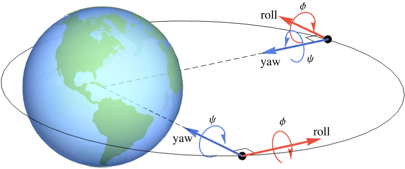
sat = StateSpaceModel[IconizedObject[«abcd»], IconizedObject[«labels»]]sr = StateResponse[{sat, {0.1, 0, 0.5, 0}}, {0, 0, 0, 0}, {t, 0, 100}];
Plot[sr, {t, 0, 100}, IconizedObject[«plotOpts»]]sspec = <|"InputModel" -> sat, "FeedbackInputs" -> {1, 2}|>;{cvs, wts} = {{(| | |
| -- | ---- |
| 10 | 0 |
| 0 | 10^2 |), (| | |
| --- | ---- |
| 0.1 | 0 |
| 0 | 0.01 |)}, {(| | | | |
| ---- | - | ---- | - |
| 10^3 | 0 | 0 | 0 |
| 0 | 1 | 0 | 0 |
| 0 | 0 | 10^3 | 0 |
| 0 | 0 | 0 | 1 |), (| | |
| - | - |
| 1 | 0 |
| 0 | 1 |)}};lqg = LQGRegulator[sspec, cvs, wts, "Data"]csys = lqg["ClosedLoopSystem"]ノイズが多い信号を生成して過程のノイズのシミュレーションを行う:
n = 100;Thread[{Range[0, n], RandomVariate[NormalDistribution[0, Sqrt[2 10^-4]], {n + 1}]}];
Plot[Subscript[u, w] = Interpolation[%, t], {t, 0, n}]Thread[{Range[0, n], RandomVariate[NormalDistribution[0, Sqrt[10^-6]], {n + 1}]}];
Plot[Subscript[y, v] = Interpolation[%, t], {t, 0, n}]sr = StateResponse[{csys, {0.1, 0, 0.5}}, {0, 0, 0, 0, Subscript[u, w], Subscript[y, v]}, {t, 0, 30}];
Table[Plot[𝓈𝓇[[1]], {t, 0, 30}, IconizedObject[«plotOpts»]], {𝓈𝓇, ({sr[[{1, 3}]], {ϕ, ψ}})}]cm = lqg["ControllerModel"]OutputResponse[cm, Join[{0, 0}, sr[[1 ;; 3]]], {t, 0, 30}];
Plot[%, {t, 0, 30}, PlotRange -> All, PlotLegends -> {"SubscriptBox[𝒯, ϕ]", "SubscriptBox[𝒯, ψ]"}]sat = StateSpaceModel[IconizedObject[«abcd»], IconizedObject[«labels»]]衛星の軌道は η 状態における初期外乱に対して不安定である:
OutputResponse[{sat, {0, 5}}, {0, 0, 0, 0}, {t, 0, 10}];
Plot[%, {t, 0, 10}, PlotRange -> All, PlotLegends -> {ζ, η, ξ}]
衛星を制御するためには,少なくとも小型ロケットエンジン  ともう一つの小型ロケットエンジンが必要である:
Grid[{#, ControllableModelQ[SystemsModelExtract[sat, #, All]]}& /@ Subsets[{1, 2, 3}, {1, 3}], Frame -> All]sspec = <|"InputModel" -> sat, "FeedbackInputs" -> {1, 2, 3}|>;cvs = {{{10^5}}, 10^-8IdentityMatrix[3]};
wts = {IdentityMatrix[6], IdentityMatrix[3]};lqg = LQGRegulator[sspec, cvs, wts, "Data"]csys = lqg["ClosedLoopSystem"]//Chopノイズがある信号を生成して過程のノイズのシミュレーションを行う:
n = 60;Thread[{Range[0, n], RandomVariate[NormalDistribution[0, Sqrt[10^-4]], {n + 1}]}];
Plot[Subscript[u, w] = Interpolation[%, t], {t, 0, n}]Table[Thread[{Range[0, n], RandomVariate[NormalDistribution[0, Sqrt[10^-4]], {n + 1}]}], 3];
Subscript[y, v] = Interpolation[#, t]& /@ %衛星の軌道は η 状態における初期外乱に対して調整されている:
or = OutputResponse[{csys, {0, 5, 0}}, Join[{0, 0, 0}, {Subscript[u, w]}, Subscript[y, v]], {t, 0, 20}];
Plot[%, {t, 0, 15}, PlotRange -> All, PlotLegends -> {ζ, η, ξ}]cm = lqg["ControllerModel"]//ChopOutputResponse[cm, Join[{0}, or], {t, 0, 20}];
Plot[%, {t, 0, 15}, PlotRange -> All, PlotLegends -> {Subscript[𝓊, 1], Subscript[𝓊, 2], Subscript[𝓊, 3]}]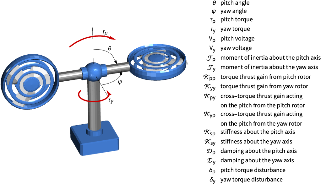
ssm = StateSpaceModel[IconizedObject[«eqns»] /. IconizedObject[«pars»], {θ[t], ψ[t], θ'[t], ψ'[t]}, {Subscript[V, p][t], Subscript[V, y][t], Subscript[δ, p][t], Subscript[δ, y][t]}, {θ[t], ψ[t]}, t, IconizedObject[«labels»]]
dssm = ToDiscreteTimeModel[ssm, τ = 0.1]//Chopピッチモーターへのステップ入力はピッチとヨーに同時に影響する:
OutputResponse[dssm, {0, 0, UnitStep[t], 0}, {t, 100}];
Table[ListStepPlot[ℴ𝓇[[1]], IconizedObject[«plotOpts»]], {ℴ𝓇, ({%, {θ, ψ}})}]OutputResponse[dssm, {0, UnitStep[t]}, {t, 10}];
Table[ListStepPlot[ℴ𝓇[[1]], IconizedObject[«plotOpts»]], {ℴ𝓇, ({%, {θ, ψ}})}]ヨーとピッチのモーター電圧に対するフィードバック入力を設定する:
sspec = <|"InputModel" -> dssm, "FeedbackInputs" -> {1, 2}|>;cvs = {(| | |
| -- | -- |
| 10 | 0 |
| 0 | 10 |), (| | |
| ----- | ----- |
| 0.025 | 0 |
| 0 | 0.025 |)};wts = {(| | | | |
| --------- | ------------- | ---------- | ---------- |
| (1/θmax2) | 0 | 0 | 0 |
| 0 | (1/0.05ϕmax2) | 0 | 0 |
| 0 | 0 | (1/θvmax2) | 0 |
| 0 | 0 | 0 | (1/ϕvmax2) |), (| | |
| --------- | --------- |
| (1/vmax2) | 0 |
| 0 | (1/vmax2) |)} /. IconizedObject[«wtspec»];lqg = LQGRegulator[sspec, cvs, wts, "Data"]csys = lqg["ClosedLoopSystem"]//Chopノイズが多い信号を2つ生成してピッチとヨーの過程ノイズのシミュレーションを行う:
n = 100;
Subscript[u, w] = RandomVariate[NormalDistribution[0, Sqrt[2 10^-5]], {2, n + 1}];
ListStepPlot[%, DataRange -> {0, n - 1}, PlotRange -> All]
ピッチおよびヨーの位置センサー用にもう2つの信号を生成してシミュレーションを行う:
Subscript[y, v] = RandomVariate[NormalDistribution[0, Sqrt[5 10^-5]], {2, n + 1}];
ListStepPlot[%, DataRange -> {0, n - 1}, PlotRange -> All]orclθ = OutputResponse[csys, Join[Subscript[u, w], ConstantArray[#, n + 1]& /@ {0, 1}, Subscript[y, v]]];
ListStepPlot[%, DataRange -> {0, 99τ}, PlotRange -> All, PlotLegends -> {θ, ψ}]orclψ = OutputResponse[csys, Join[Subscript[u, w], ConstantArray[#, n + 1]& /@ {1, 0}, Subscript[y, v]]];
ListStepPlot[%, DataRange -> {0, 99τ}, PlotRange -> All, PlotLegends -> {θ, ψ}]cm = lqg["ControllerModel"]OutputResponse[cm, ArrayPad[#, {{2, 0}, 0}]]& /@ {orclθ, orclψ};
Table[ListStepPlot[ℴ𝓇[[1]], IconizedObject[«plotOpts»]], {ℴ𝓇, ({%, IconizedObject[«plotLabels»]})}]海洋系 (1)
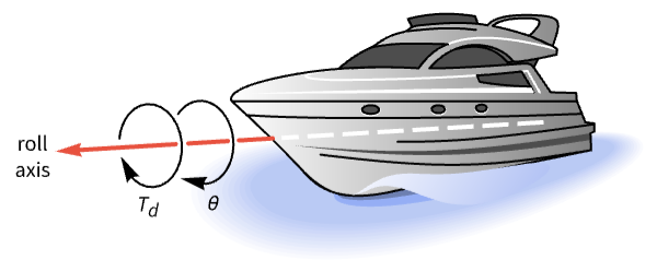
roll = TransferFunctionModel[{{{2.25}}, 2.25 + 0.5*s + s^2}, s];OutputResponse[roll, UnitStep[t], {t, 0, 15}];
Plot[%, {t, 0, 15}, PlotRange -> All]ボード線図を見ると振動の原因となっている低周波数応答のピークが顕著である:
olfr = BodePlot[roll, IconizedObject[«plotOpts»]]roll = StateSpaceModel[roll, SystemsModelLabels -> {Subscript[𝒯, d], θ, {θ, ω}}]{cvs, wts} = {{{{}}, {{10^2}}}, {50IdentityMatrix[2], {{1}}}};
lqg = LQGRegulator[roll, cvs, wts, "Data"]csys = lqg["ClosedLoopSystem"]ピッチ測定におけるノイズのシミュレーションのためのノイズの多い信号を生成する:
n = 15;Thread[{Range[0, n], RandomVariate[NormalDistribution[0, 2Sqrt[10^-2]], {n + 1}]}];
Plot[Subscript[y, v] = Interpolation[%, t], {t, 0, n}]or = OutputResponse[csys, {Subscript[y, v] + UnitStep[t], 0}, {t, 0, 15}];
Plot[%, {t, 0, 15}, PlotRange -> All]開ループ系と閉ループ系の周波数応答はピークが減衰されていることを示している:
BodePlot[{roll, csys}, IconizedObject[«plotOpts»]]cm = lqg["ControllerModel"]OutputResponse[cm, or, {t, 0, 15}];
Plot[%, {t, 0, 15}, PlotRange -> All]生物学系 (1)
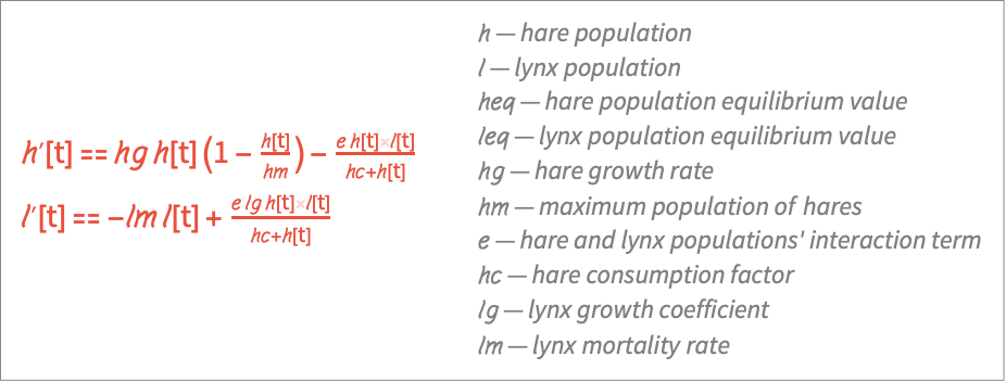
nssm = NonlinearStateSpaceModel[IconizedObject[«eqns»], {{𝒽[t], 𝒽ℯ𝓆}, {ℓ[t], ℓℯ𝓆}}, {𝒽ℊ[t], ℓℊ[t]}, {𝒽[t], ℓ[t]}, t] /. IconizedObject[«pars»]OutputResponse[{nssm, {23, 20}}, {0, 0}, {t, 0, 40}];
Plot[%, {t, 0, 40}, IconizedObject[«plotOpts»]]cvs = {{{}}, 10^-2DiagonalMatrix[{1, 1}]};wts = {DiagonalMatrix[{5, 5}], DiagonalMatrix[0.1{1, 1}]};nssm = NonlinearStateSpaceModel[nssm, Automatic, Automatic, Automatic, None];lqg = LQGRegulator[nssm, cvs, wts, "Data"]csys = lqg["ClosedLoopSystem"]//FullSimplifyn = 120;Thread[{Range[0, n], RandomVariate[NormalDistribution[0, Sqrt[1.5]], {n + 1}]}];
Plot[Subscript[y, v] = Interpolation[%, t], {t, 0, n}]or = OutputResponse[{csys, {23, 20}}, {Subscript[y, v], 0, 0}, {t, 0, 120}];
Plot[%, {t, 0, 120}, IconizedObject[«plotOpts»]]ParametricPlot[or, {t, 0, 60}, PlotRange -> All, AxesOrigin -> {0, 0}]cm = lqg["ControllerModel"]//Simplify制御努力からノウサギとオオヤマネコの成長率の平衡値が明らかになる:
OutputResponse[cm, Join[{0, 0}, or], {t, 0, 120}];
Plot[%, {t, 0, 1}, PlotRange -> All, PlotLegends -> {𝓇, 𝒷}]
経済系 (1)
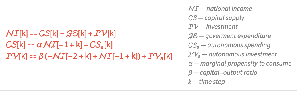
dssm = StateSpaceModel[IconizedObject[«eqns»] /. IconizedObject[«pars»], {ℐ𝒱[k], 𝒞𝒮[k], 𝒩ℐ[k]}, {𝒢ℰ[k], Subscript[𝒞𝒮, a][k], Subscript[ℐ𝒱, a][k]}, 𝒩ℐ[k], k, DescriptorStateSpace -> True]n = 50;
OutputResponse[dssm, Table[{0, 10, 0}, n]];
ListStepPlot[%, PlotRange -> All]cvs = {{{}}, {{10^-6}}};wts = {DiagonalMatrix[{1, 10, 1, 10^2, 1}], DiagonalMatrix[{0.1, 0.5, 1}]};lqg = LQGRegulator[dssm, cvs, wts, "Data"]csys = lqg[{"ClosedLoopSystem", <|"Merge" -> True|>}]Subscript[y, v] = RandomVariate[NormalDistribution[0, Sqrt[10^-6]], {1, n}];
ListStepPlot[%, DataRange -> {0, n - 1}, PlotRange -> All]or = OutputResponse[{csys, {0, 10, 1}}, Join[ConstantArray[#, n]& /@ {0, 0, 0}, Subscript[y, v]]];
ListStepPlot[%, DataRange -> {0, n - 1}, PlotRange -> All]cm = lqg[{"ControllerModel", <|"Merge" -> True|>}]//ChopOutputResponse[cm, or];
ListStepPlot[%, DataRange -> {0, n - 1}, IconizedObject[«plotOpts»]]化学系 (1)
 におけるCSTRの動作を改善する:
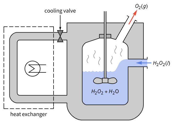
cstr = StateSpaceModel[IconizedObject[«abcd»], IconizedObject[«labels»]]PoleZeroPlot[cstr]olor = OutputResponse[{cstr, {0, -1}}, {0, 0}, {t, 0, 200}];
Plot[%, {t, 0, 200}, PlotRange -> All]sspec = <|"InputModel" -> cstr, "FeedbackInputs" -> 1|>;
{cvs, wts} = {{(10^-2), (10^-3)}, {(| | |
| ---- | ---- |
| 10^3 | 0 |
| 0 | 10^3 |), (1)}};lqg = LQGRegulator[sspec, cvs, wts, "Data"]csys = lqg["ClosedLoopSystem"]PoleZeroPlot[csys]ノイズのある信号を生成して過程のノイズのシミュレーションを行う:
Subscript[u, w] = With[{n = 200}, Interpolation[Thread[{Range[0, n],
RandomVariate[NormalDistribution[0, Sqrt[0.05]], {n + 1}]}], t]]sr = StateResponse[{csys, {0, -1}}, {0, Subscript[u, w], 0}, {t, 0, 200}];
Plot[{olor, sr[[2]]}, {t, 0, 200}, IconizedObject[«plotOpts»]]cm = lqg["ControllerModel"]OutputResponse[cm, sr[[1 ;; 2]], {t, 0, 200}];
Plot[%, {t, 0, 200}, PlotRange -> All]電気系 (1)
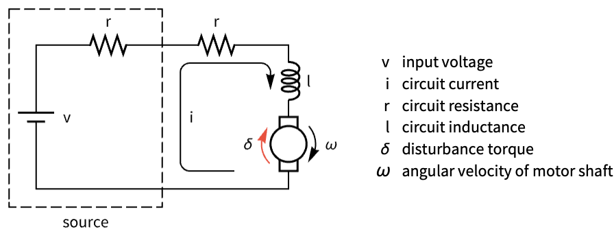
dcm = StateSpaceModel[IconizedObject[«eqns»] /. IconizedObject[«pars»], {ω[t], i[t]}, {v[t], δ[t]}, ω[t], t, IconizedObject[«labels»]]ddcm = ToDiscreteTimeModel[dcm, τ = 0.1]OutputResponse[ddcm, Table[{0, -10^-2}, 15]];
ListStepPlot[%, DataRange -> {0, 14τ}, PlotRange -> All]sspec = <|"InputModel" -> ddcm, "FeedbackInputs" -> 1, "TrackedOutputs" -> 1|>;
{cvs, wts} = {{{{10^4}}, {{10^-2}}}, {(| | | |
| ---- | - | - |
| 0.1 | 0 | 0 |
| 0 | 1 | 0 |
| 0 | 0 | 1 |), ((1/5^2))}};lqg = LQGRegulator[sspec, cvs, wts, "Data"]csys = lqg[{"ClosedLoopSystem", <|"Merged" -> True|>}]//Chopノイズがある信号を生成して過程ノイズのシミュレーションを行う:
n = 100;Subscript[u, w] = RandomVariate[NormalDistribution[0, Sqrt[10^-8]], n];
ListStepPlot[%, DataRange -> {0, n - 1}, PlotRange -> All]Subscript[y, v] = RandomVariate[NormalDistribution[0, Sqrt[2 10^-6]], n];
ListStepPlot[%, DataRange -> {0, n - 1}, PlotRange -> All]ref = 50;
(inps = Join[{Subscript[u, w]}, {ConstantArray[50, n]}, {Subscript[y, v]}])//Shortor = OutputResponse[csys, inps];
Show[ListStepPlot[or, DataRange -> {0, 99 τ}, IconizedObject[«plotOpts»]], Plot[ref, {x, 0, τ (n - 1)}, IconizedObject[«plotOpts»]]]cm = lqg[{"ControllerModel", <|"Merge" -> True|>}]Short[cinps = Join[{ConstantArray[ref, n]}, or]]
OutputResponse[cm, cinps];
ListStepPlot[%, DataRange -> {0, τ (n - 1)}, PlotRange -> All]
特性と関係 (8)
ssm = StateSpaceModel[{{{0, 1}, {-3, -0.5}}, {{0}, {1}}, {{1, 0}}, {{0}}}, SamplingPeriod -> None,
SystemsModelLabels -> None];
{cvs, wts} = {{{{}}, (0.01)}, {(| | |
| - | - |
| 1 | 0 |
| 0 | 1 |), (0.1)}};lqgp = LQGRegulator[ssm, cvs, wts, "ClosedLoopPoles"]KalmanEstimator[{ssm, 1, 1}, cvs];
kep = Eigenvalues[First[Normal[%]]]lqrp = LQRegulatorGains[ssm, wts, "ClosedLoopPoles"]ContainsExactly[Join[kep, lqrp], lqgp, SameTest -> (Chop[#1 - #2] == 0.&)]外因性入力  から測定値
 への閉ループは出力フィードバック系である:
sspec = <|"InputModel" -> StateSpaceModel[{{{0, -6}, {1, -5}}, {{1, -6}, {1, -3}}, {{0, 1}}, {{0, 1}}},
SamplingPeriod -> None, SystemsModelLabels -> None], "FeedbackInputs" -> 2|>;
{cvs, wts} = {{(1), (0.5)}, {(| | |
| - | - |
| 1 | 0 |
| 0 | 1 |), (1.0)}};lqg = LQGRegulator[sspec, cvs, wts, "Data"]erm = lqg["EstimatorRegulatorModel"]{sum, comp} = Table[TransferFunctionModel[{i}], {i, {{1, 1}, {1, -1}}}]


SystemsConnectionsModel[{sspec["InputModel"], erm, comp, sum}, IconizedObject[«conxs»]];
csys1 = SystemsModelMerge[%]csys2 = lqg["ClosedLoopSystem"]Normal[csys1] == Normal[csys2]

SystemsModelExtract[csys2, 2]測定ノイズ  から測定値
 への閉ループは単位フィードバック系である:
ssm = StateSpaceModel[{{{0, 1}, {-1., 2.}}, {{0}, {1.}}, {{1., 0}}, {{0}}}, SamplingPeriod -> None,
SystemsModelLabels -> None];
{cvs, wts} = {{{{}}, (10^-2)}, {(| | |
| ---- | ---- |
| 10^2 | 0 |
| 0 | 10^4 |), (1)}};lqg = LQGRegulator[ssm, cvs, wts, "Data"]

SystemsModelExtract[lqg["ClosedLoopSystem"], 2];
csys1 = TransferFunctionModel[%]
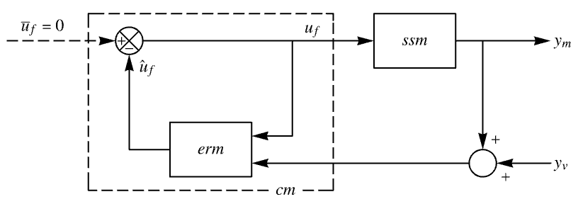
cm = SystemsModelDelete[lqg["ControllerModel"], 1]

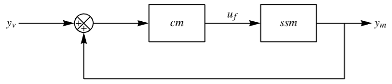
SystemsModelFeedbackConnect[SystemsModelSeriesConnect[cm, ssm], {1, 1, 1}]
csys2 = TransferFunctionModel[%]Chop[Together[csys1[s] - csys2[s]], 10^-5]LQGRegulatorはEstimatorRegulatorを使って組み立てられる:
ssm = StateSpaceModel[{{{-2.9, 5}, {0.8, -1.3}}, {{-1.1}, {0}}, {{1, 0}}, {{0.1}}}, SamplingPeriod -> 1,
SystemsModelLabels -> None]{w, v} = {{{}}, (0.1)};
ℓ = LQEstimatorGains[{ssm, 1, 1}, {w, v}]{q, r} = {(| | |
| ---- | ---- |
| 10^4 | 0 |
| 0 | 10^2 |), (10^2)};
κ = LQRegulatorGains[ssm, {q, r}]EstimatorRegulatorを使ってLQGRegulatorを組み立てる:
EstimatorRegulator[ssm, {ℓ, κ}]LQGRegulatorは同じ結果を与える:
LQGRegulator[ssm, {w, v}, {q, r}]Kalman推定器と最適状態フィードバックゲインモデルから線形二次ガウス調整器を構築する:
sspec = <|"InputModel" -> StateSpaceModel[{{{-1, 0}, {0, -2}}, {{0.1, -0.2}, {0, -0.1}}, {{2, 0}}, {{0, 0}}},
SamplingPeriod -> None, SystemsModelLabels -> None], "FeedbackInputs" -> 2|>;
{cvs, wts} = {{(10^-4), (10^-2)}, {(| | |
| ----- | ----- |
| 0.001 | 0 |
| 0 | 0.001 |), (0.1)}};est = KalmanEstimator[{sspec["InputModel"], 1, 2}, cvs]gm = LQRegulatorGains[sspec, wts, "FeedbackGainsModel"]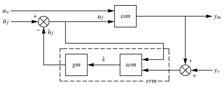
sem = SystemsModelExtract[est, All, {1, 2}];
erm = SystemsModelSeriesConnect[sem, gm]LQGRegulatorも同じ結果を与える:
LQGRegulator[sspec, cvs, wts]LQRコントローラのパフォーマンスは同等のLQGコントローラのそれよりも上である:
sspec = <|"InputModel" -> StateSpaceModel[{{{0, 1, 0}, {0, -0.875, -20}, {0, 0, -50}}, {{0, 0}, {0, 0}, {50, 50}},
{{1, 0, 0}}, {{0, 0}}}, SamplingPeriod -> None, SystemsModelLabels -> None], "FeedbackInputs" -> 1|>;
{cvs, wts} = {{(10^-3), (10^-2)}, {(| | | |
| --- | --- | --- |
| 100 | 0 | 0 |
| 0 | 0.1 | 0 |
| 0 | 0 | 0.1 |), (100)}};csyslqr = LQRegulatorGains[sspec, wts, "ClosedLoopSystem"]csyslqg = LQGRegulator[sspec, cvs, wts, "ClosedLoopSystem"]orLQR = OutputResponse[{csyslqr, PadRight[{1}, 3]}, {0, 0}, {t, 0, 5}];
orLQG = OutputResponse[{csyslqg, PadRight[{1}, 6]}, {0, 0}, {t, 0, 5}];
Plot[{orLQR, orLQG}, {t, 0, 5}, IconizedObject[«plotOpts»]]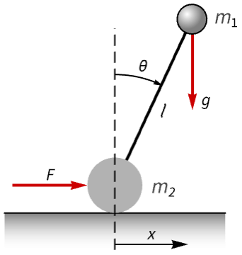
nssm = NonlinearStateSpaceModel[IconizedObject[«eqns»], {{θ[t], π}, {x[t], 0}}, {F[t], δ[t]}, {θ[t], x[t]}, t]//Simplify;
nssm = NonlinearStateSpaceModel[nssm, Automatic, Automatic, Automatic, None]sspec = <|"InputModel" -> nssm /. IconizedObject[«pars»], "FeedbackInputs" -> 1|>;cvs = {{{1}}, DiagonalMatrix[{1, 1}]};
wts = {DiagonalMatrix[{50, 10, 100, 50}], {{0.5}}};lqg = LQGRegulator[sspec, cvs, wts, "Data"]lqr = LQRegulatorGains[sspec, wts, "Data"]csyslqg = lqg[{"ClosedLoopSystem", <|"InputModel" -> nssm /. IconizedObject[«pars»]|>}];
csyslqgP = lqg[{"ClosedLoopSystem", <|"InputModel" -> nssm /. IconizedObject[«parsP»]|>}];Head /@ {csyslqg, csyslqgP}csyslqr = lqr[{"ClosedLoopSystem", <|"InputModel" -> nssm /. IconizedObject[«pars»]|>}];
csyslqrP = lqr[{"ClosedLoopSystem", <|"InputModel" -> nssm /. IconizedObject[«parsP»]|>}];Thread[Table[OutputResponse[sys, {0, 0.5Sin[2t]}, {t, 0, 60}], {sys, {csyslqg, csyslqgP}}]];{Plot[Evaluate[%[[1]]], {t, 0, 45}, IconizedObject[«plotOpts»]], Plot[Evaluate[%[[2]]], {t, 0, 45}, IconizedObject[«plotOpts»]]}LQRは,名目応答と摂動応答の間の変動が少なく,より強力である:
Thread[Table[OutputResponse[sys, {0, 0.5Sin[2t]}, {t, 0, 60}], {sys, {csyslqr, csyslqrP}}]];
{Plot[Evaluate[%[[1]]], {t, 0, 45}, IconizedObject[«plotOpts»]], Plot[Evaluate[%[[2]]], {t, 0, 45}, IconizedObject[«plotOpts»]]}
LQGコントローラのパフォーマンスは共分散行列を調整することで改善できる:
sspec = <|"InputModel" -> StateSpaceModel[{{{0, 1, 0}, {0, -0.875, -20}, {0, 0, -50}}, {{0, 0}, {0, 0}, {50, 50}},
{{1, 0, 0}}, {{0, 0}}}, SamplingPeriod -> None, SystemsModelLabels -> None], "FeedbackInputs" -> 1|>;
{{w1, v1}, wts} = {{(10^-3), (10^-2)}, {(| | | |
| --- | --- | --- |
| 100 | 0 | 0 |
| 0 | 0.1 | 0 |
| 0 | 0 | 0.1 |), (100)}};csys1 = LQGRegulator[sspec, {w1, v1}, wts, "ClosedLoopSystem"]{w2, v2} = {10^8w1, 10^-4v1};csys2 = LQGRegulator[sspec, {w2, v2}, wts, "ClosedLoopSystem"]Table[OutputResponse[{csys, PadRight[{1}, 6]}, {0, 0}, {t, 0, 5}][[1]], {csys, {csys1, csys2}}];
Plot[%, {t, 0, 5}, PlotRange -> All, PlotLegends -> {"{w1,v1}", "{w2,v2}"}]テキスト
Wolfram Research (2010), LQGRegulator, Wolfram言語関数, https://reference.wolfram.com/language/ref/LQGRegulator.html (2023年に更新).
CMS
Wolfram Language. 2010. "LQGRegulator." Wolfram Language & System Documentation Center. Wolfram Research. Last Modified 2023. https://reference.wolfram.com/language/ref/LQGRegulator.html.
APA
Wolfram Language. (2010). LQGRegulator. Wolfram Language & System Documentation Center. Retrieved from https://reference.wolfram.com/language/ref/LQGRegulator.html