Enable JavaScript to interact with content and submit forms on Wolfram websites. Learn how

UnitRootTest

UnitRootTest[data]

测试数据是否来自具有单位根的自回归时间序列过程.

UnitRootTest[data,model,"property"]

返回给定模型的 "property" 值.

更多信息和选项

UnitRootTest 对时间序列 data 执行假设检验，其中零假设为满足 AR 模型的时间序列在相应的传递函数的分母中有一个单位根，而置换假设则相反.
拒绝零假设允许去掉趋势的 data 可能来自平稳时间序列的结论.
默认情况下，返回概率值或者值.
较小的值表明单位根的存在是不可能的.
data 可以是数值列表 {x₁,x₂,…,x_n} 或者 TemporalData 对象.
model 允许模型指定，其中是常量偏移，是线性 drift，而是AR 模型的阶数.
可以使用下列 model 指定：
Automatic 和

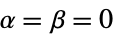
r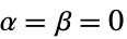

"Constant" 和

"Drift"

{"Constant",r}

{"Drift", r} 一般情况
UnitRootTest[data] 将选择 Dickey–Fuller F 检验，其中并且 .
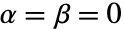UnitRootTest[data,model,All] 将选项所有应用于 data 和 model 的检验.
UnitRootTest[data,model,"test"] 报告值，根据 "test".
可以使用下列检验：

	"DickeyFullerF"	基于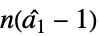
	"DickeyFullerT"	基于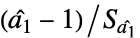
	"PhillipsPerronF"	经过调整的 Dickey–Fuller F 检验
	"PhillipsPerronT"	经过调整的 Dickey–Fuller T 检验

UnitRootTest[data,model,"HypothesisTestData"] 返回 HypothesisTestData 对象 htd，它可以用于使用格式 htd["property"] 提取额外检验结果和属性.
UnitRootTest[data,model,"property"] 用于直接给出 "property" 的值.
与检验结果报告相关的属性包括：

	"AllTests"	所有可用检验列表
	"AutomaticTest"	如果使用 Automatic 所选的检验
	"PValue"	值检验
	"PValueTable"	值的格式化表格
	"ShortTestConclusion"	检验结论的简单说明
	"TestConclusion"	检验结论的说明
	"TestData"	检验统计量与值的数对列表
	"TestDataTable"	值与检验统计量的格式化表格
	"TestStatistic"	检验统计量的列表
	"TestStatisticTable"	检验统计量的格式化表格

可以使用下列选项：
SignificanceLevel 0.05 诊断和报告的截止值
对于单位根检验，所选择的截止值使得仅在时被拒绝. 用于 "TestConclusion" 和 "ShortTestConclusion" 性质的值由 SignificanceLevel 选项控制. 默认情况下，设置为 0.05.

范例

打开所有单元关闭所有单元

基本范例 (1)

测试时间序列是否有单位根：

数据来自弱平稳过程：

范围 (17)

检验 (13)

对单位根，测试时间序列数据：

当单位根出现时，值通常较大：

当单位根不出现时，值通常较小：

测试单位根，零假设为内在模型是 ARProcess[2]:

把模型设为 Automatic 等价于假定内在 ARProcess[1]:

考虑内在非零均值，测试单位根：

考虑非零均值，假定内在 ARProcess[3]:

假定非零均值和确定性趋势：

假定非零均值、确定性趋势和内在 ARProcess[3]:

执行单位根的特定测试：

可以同时执行任意次数的测试：

使用 Automatic 应用 Dickey–Fuller F 测试：

属性 "AutomaticTest" 可用以确定选择何种测试：

同时执行对数据合适的测试：

使用属性 "AllTests" 以识别使用何种测试：

创建 HypothesisTestData 对象，用于重复属性提取：

可用于提取的属性：

从 HypothesisTestData 对象提取某些属性：

来自 "DickeyFullerT" 检验的值和检验统计量：

同时提取任意数目的属性：

来自 Dickey–Fuller F 检验的值和检验统计量：

报告 (4)

将选中的检验结果制作表格：

所有合适的检验结果的完全表格：

选中的检验结果组成的表格：

从检验表格获取项目，实现自定义报告：

值都在 0.05 之上，因此没有足够证据在该水平拒绝：

对于一个检验或一组检验，将值制作表格：

来自表格的值：

来自所有合适的检验的值表格：

来自检验的子集的值组成的表格：

从一个检验或者一组检验报告检验统计量：

来自表格的检验统计量：

来自所有合适的检验的检验统计量的表格：

选项 (1)

SignificanceLevel (1)

用于 "TestConclusion" 和 "ShortTestConclusion" 的显著性水平：

应用 (3)

记录澳大利亚悉尼 47 年内最大日降雨量. 令人感兴趣的是一个简单的自回归模型是否可以对该数据建模：

数据明显具有非零均值：

使用 Schwert 定理选择内在 ARProcess 的阶数：

这是单位根的证据，表明一个简单的 ARProcess 不是一个正确的模型：

考虑美国商业航空公司1937年至1960年的年营业收入（以百万计）：

用 UnitRootTest 来确认这个趋势：

去除线性趋势似乎已足够：

对时间序列做 ARIMAProcess 拟合：

用拟合模型预测未来10年的营业收入：

预测 SP500 指数:

使用单位根检验判断趋势的存在：

拟合具有非零积分阶数的 ARIMA：

求下一个月的预测值：

可能存在的问题 (2)

Phillips–Perron 检验局限于ARProcess[1] 模型：

使用 Dickey–Fuller 类型检验来测试较高的阶数：

UnitRootTest 对于不规则采样数据失效：

只使用数值：

或者设置 TemporalRegularity 为真：

巧妙范例 (2)

对于样本量100，模拟 Dickey–Fuller T 分布的近似：

第一组模拟数据集的检验统计量和值：

使用模拟分布给出相似的结果：

在零假设下，某些检验统计量的近似分布：

顶部