Linear Optimization
| Introduction | Application Examples of Linear Optimization |
| The LinearOptimization Function | Algorithms for Linear Optimization |
| Examples | References |
| Importing Large Datasets and Solving Large-Scale Problems |
Introduction
Linear optimization problems are defined as problems where the objective function and constraints are all linear.
The Wolfram Language has a collection of algorithms for solving linear optimization problems with real variables, accessed via LinearOptimization, FindMinimum, FindMaximum, NMinimize, NMaximize, Minimize and Maximize. LinearOptimization gives direct access to linear optimization algorithms, provides the most flexibility for specifying the methods used, and is the most efficient for large-scale problems. FindMinimum, FindMaximum, NMinimize, NMaximize, Minimize and Maximize are convenient for solving linear optimization problems in equation and inequality form.
The LinearOptimization Function
LinearOptimization is the main function for linear optimization with the most flexibility for specifying the methods used, and is the most efficient for large-scale problems.
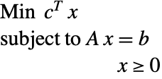
Linear optimization finds ![]() that solves the primal problem:
that solves the primal problem:
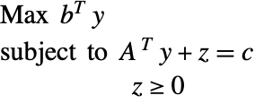
The Lagrangian dual problem for linear optimization is given by:
The following options are accepted:
option name | default value | |
| Method | Automatic | method used to solve the linear optimization problem |
| Tolerance | Automatic | convergence tolerance |
| MaxIterations | Automatic | maximum number of iterations to use |
| PerformanceGoal | $PerformanceGoal | aspects of performance to try to optimize |
| WorkingPrecision | Automatic | precision to be used in internal computations |
Options for LinearOptimization
The Method option specifies the algorithm used to solve the linear optimization problem. Possible values are Automatic, "Simplex", "RevisedSimplex", "InteriorPoint", "CLP", "MOSEK" and "Gurobi". The default is Automatic, which automatically chooses from the other methods based on the problem size and precision.
The Tolerance option specifies the convergence tolerance.
With WorkingPrecision->Automatic, the precision is taken automatically from the precision of the input arguments unless a method is specified that only works with machine precision, in which case machine precision is used.
There are a number of solution properties that can be accessed through the LinearOptimization function:
| "PrimalMinimizer" | { | A list of variable values that minimize the objective function |
| "PrimalMinimizerRules" | {v1 | values for the variables vars={v1,…} that minimize |
| "PrimalMinimizerVector" | x* | the vector that minimizes |
| "PrimalMinimumValue" | the minimum value | |
| "DualMaximizer" | the vector that maximizes | |
| "DualMaximumValue" | the dual maximum value | |
| "DualityGap" | the difference between the dual and primal optimal values (0 because of strong duality) | |
| "Slack" | the constraint slack vector | |
| "ConstraintSensitivity" | sensitivity of | |
| "ObjectiveVector" | the linear objective vector | |
| "LinearInequalityConstraints" | the linear inequality constraint matrix and vector | |
| "LinearEqualityConstraints" | the linear equality constraint matrix and vector | |
| {"prop1","prop2",...} | | several solution properties |
Solution properties for LinearOptimization.
Examples
Difference between Interior Point and Simplex and/or Revised Simplex
The simplex and revised simplex algorithms solve a linear optimization problem by moving along the edges of the polytope defined by the constraints, from vertices to vertices with successively smaller values of the objective function, until the minimum is reached. The Wolfram Language's implementation of these algorithms uses dense linear algebra. A unique feature of the implementation is that it is possible to solve exact/extended precision problems. Therefore these methods are suitable for small-sized problems for which non-machine-number results are needed, or a solution on the vertex is desirable.
Interior point algorithms for linear optimization, loosely speaking, iterate from the interior of the polytope defined by the constraints. They get closer to the solution very quickly, but unlike the simplex/revised simplex algorithms, do not find the solution exactly. The Wolfram Language's implementation of an interior point algorithm uses machine-precision sparse linear algebra. Therefore for large-scale machine-precision linear optimization problems, the interior point method is more efficient and should be used.
Finding Dual Variables
Given the general linear optimization problem
It is useful to know solutions for both for some applications.
The relationship between the solutions of the primal and dual problems is given by the following table.
if the primal is | then the dual problem is |
| feasible | feasible |
| unbounded | infeasible or unbounded |
| infeasible | unbounded or infeasible |
When both problems are feasible, then the optimal values of (P) and (D) are the same, and the following complementary conditions hold for the primal solution ![]() and dual solution
and dual solution ![]() .
.
The dual maximizer can be obtained from LinearOptimization using the "DualMaximizer" solution property.
Dealing with Infeasibility and Unboundedness in the Interior Point Method
The primal-dual interior point method is designed for feasible problems; for infeasible/unbounded problems it will diverge, and with the current implementation, it is difficult to find out if the divergence is due to infeasibility or unboundedness.
The Method Options of "InteriorPoint"
"TreatDenseColumn" is a method option of "InteriorPoint" that decides if dense columns are to be treated separately. Dense columns are columns of the constraint matrix that have many nonzero elements. By default, this method option has the value Automatic, and dense columns are treated separately.
Importing Large Datasets and Solving Large-Scale Problems
A commonly used format for documenting linear optimization problems is the Mathematical Programming System (MPS) format. This is a text format consisting of a number of sections.
Importing MPS Formatted Files in Equation Form
The Wolfram Language is able to import MPS formatted files. By default, Import of MPS data returns a linear optimization problem in equation form, which can then be solved using LinearOptimization, Minimize or NMinimize.
Large-Scale Problems: Importing in Matrix and Vector Form
For large-scale problems, it is more efficient to import the MPS data file and represent the linear optimization using matrices and vectors, then solve using LinearOptimization.
Free Formatted MPS Files
Standard MPS formatted files use a fixed format, where each field occupies a strictly fixed character position. However some modeling systems output MPS files with a free format, where fields are positioned freely. For such files, the option "FreeFormat"->True can be specified for Import.
Linear Optimization Test Problems
Through the ExampleData function, all NetLib linear optimization test problems can be accessed.
Application Examples of Linear Optimization
L1-Norm Minimization
It is possible to solve an ![]() minimization problem
minimization problem
by turning the system into a linear optimization problem
Design of Optimal Truss
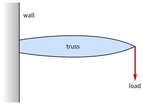
The example is adopted from [2]. The aim is to design an anchor that uses as little material as possible to support a load.
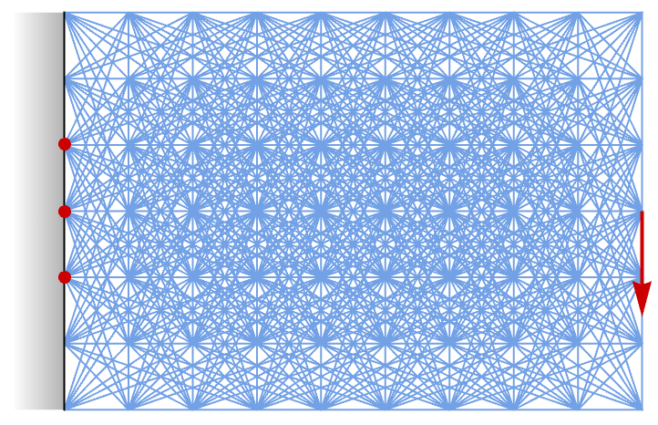
This problem can be modeled by discretizing and simulating it using nodes and links. The modeling process is illustrated using the following figure. Here a grid of 7×10 nodes is generated. Each node is then connected by a link to all other nodes that are of Manhattan distance of less than or equal to three. The three red nodes are assumed to be fixed to the wall, while on all other nodes, compression and tension forces must balance.
Each link represents a rigid rod that has a thickness, with its weight proportional to the force on it and its length. The aim is to minimize the total material used, which is
Hence mathematically this is a linearly constrained minimization problem, with objective function a sum of absolute values of linear functions.
The absolute values ![]() in the objective function can be replaced by breaking down
in the objective function can be replaced by breaking down ![]() into a combination of compression and tension forces, with each non-negative. Thus assume
into a combination of compression and tension forces, with each non-negative. Thus assume ![]() is the set of links,
is the set of links, ![]() the set of nodes,
the set of nodes, ![]() the length of the link between nodes
the length of the link between nodes ![]() and
and ![]() , and
, and ![]() and
and ![]() the compression and tension forces on the link; then the above model can be converted to a linear optimization problem.
the compression and tension forces on the link; then the above model can be converted to a linear optimization problem.
Algorithms for Linear Optimization
Simplex and Revised Simplex Algorithms
The simplex and revised simplex algorithms solve linear optimization problems by constructing a feasible solution at a vertex of the polytope defined by the constraints, and then moving along the edges of the polytope to vertices with successively smaller values of the objective function until the minimum is reached.
Although the sparse implementation of simplex and revised algorithms is quite efficient in practice, and is guaranteed to find the global optimum, the algorithms have a poor worst-case behavior: it is possible to construct a linear optimization problem for which the simplex or revised simplex method takes a number of steps exponential in the problem size.
The Wolfram Language implements simplex and revised simplex algorithms using dense linear algebra. The unique feature of this implementation is that it is possible to solve exact/extended precision problems. Therefore these methods are more suitable for small-sized problems for which non-machine number results are needed.
Interior Point Algorithm
Although the simplex and revised simplex algorithms can be quite efficient on average, they have a poor worst-case behavior. It is possible to construct a linear optimization problem for which the simplex or revised simplex methods take a number of steps exponential in the problem size. The interior point algorithm, however, has been proven to converge in a number of steps that are polynomial in the problem size.
Furthermore, the Wolfram Language simplex and revised simplex implementation use dense linear algebra, while its interior point implementation uses machine-number sparse linear algebra. Therefore for large-scale, machine-number linear optimization problems, the interior point method is more efficient and should be used.
Interior Point Formulation
Consider the standardized linear optimization problem
where ![]() ,
, ![]() ,
, ![]() . This problem can be solved using a barrier function formulation to deal with the positive constraints.
. This problem can be solved using a barrier function formulation to deal with the positive constraints.
The first-order necessary condition for the preceding problem gives:
Let ![]() denote the diagonal matrix made of the vector
denote the diagonal matrix made of the vector ![]() , and
, and ![]() .
.
This is a set of ![]() linear/nonlinear equations with constraints. It can be solved using Newton's method
linear/nonlinear equations with constraints. It can be solved using Newton's method
One way to solve this linear system is to use Gaussian elimination to simplify the matrix into block triangular form.
To solve this block triangular matrix, the so-called normal system can be solved, with the matrix in this normal system:
This matrix is positive definite, but becomes very ill-conditioned as the solution is approached. Thus numerical techniques are used to stabilize the solution process, and typically the interior point method can only be expected to solve the problem to a tolerance of about ![]() , with tolerance explained in "Convergence Tolerance". The Wolfram Language uses Mehrotra's predictor-corrector scheme [1].
, with tolerance explained in "Convergence Tolerance". The Wolfram Language uses Mehrotra's predictor-corrector scheme [1].
Convergence Tolerance
General linear optimization problems are first converted to the standard form
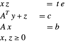
The convergence criterion for the interior point algorithm is
with the tolerance set, by default, to ![]() .
.


