带有不确定性的回归
带有不确定性的回归


n = 2500;
ys = RandomReal[{-10.5, 10.5}, n];
rs = RandomVariate[NormalDistribution[], n];
xs = 5Sin[3ys / 4] + ys / 2 + rs / 2;
ys = ys + rs * Sin[ys / 4] / 2;
plot = ListPlot[Transpose[{xs, ys}], PlotRange -> All]
当给出输入值 x(其中,x 和 y 可以是标量、向量、矩阵等),普通递归网络预测单个 y 值. 密度网络的基本思想是计算 y 值的分布. 网络按 x 函数学习该分布的参数. 混合密度网络学习简单分布的混合. 例如,我们使用 6 个高斯混合.
构建一个接受输入数并使用多层感知产生三个独立向量的网络. 每个向量包含 6 个数字表示 6 个独立高斯分量的参数. 这些向量的两个("mean" 和 "stddev")表示高斯的平均和标准差. 最终向量 ("weight") 是概率向量表示如何混合这 6 个高斯产生单个分布. 注意,我们使用 Exp 激活确保标准差是正的,并使用 SoftmaxLayer 确保权和为 1:
nmix = 6;
parameterNet = NetGraph[<|
	"mlp" -> {50, Ramp, 50, Tanh}, "mean" -> nmix,
	"stddev" -> {nmix, Exp},
	"weight" -> {nmix, SoftmaxLayer[]}|>,
	{"mlp" -> "mean" -> NetPort["mean"], "mlp" -> "stddev" -> NetPort["stddev"], "mlp" -> "weight" -> NetPort["weight"]}, "Input" -> {}]
接下来,我们训练一个更大的网络培训这个参数网络. 这个更大的网络从我们的数据分布中接受实际 x 和 y 值并计算负的对数似然性,它是度量我们参数网络表示的模型中数据的可能性. 通过最小化负的对数似然性,我们有效地最大化实际数据的似然性,它是训练概率模型的常用技术.
gaussianLikelihood[y_, μ_, σ_] := PDF[NormalDistribution[μ, σ], y];
trainingNet = NetGraph[
	<|"params" -> parameterNet, "repy" -> ReplicateLayer[nmix],
	"lhood" -> ThreadingLayer[gaussianLikelihood],
	"wsum" -> DotLayer[], "neglog" -> ElementwiseLayer[-Log[#]&]|>,
	{NetPort["x"] -> "params", NetPort["y"] -> "repy",
	{"repy", NetPort["params", "mean"], NetPort["params", "stddev"]} -> "lhood",
{"lhood", NetPort["params", "weight"]} -> "wsum" -> "neglog" -> NetPort["Loss"]}]用 NetInitialize 随机初始化网络并把之应用于单个输入:
NetInitialize[trainingNet][<|"x" -> 5, "y" -> 8|>]我们现在可以训练模型,这对应于同时最大化生成数据集中每个点的模型的似然性. 训练完成后,我们将从训练网内提取参数网. 我们不再需要训练网络,因为我们不需要再次计算训练数据的负对数-似然性. 当给定 x 值时,参数网产生均值、标准偏差和权重的关联.
Train the net with用 NetTrain 训练网络 3000 轮. 指明 LossFunction"Loss" 以确保 NetTrain 直接从 "Loss" 端口最小化输出,而不是试着自动附加损失层:
results = NetTrain[trainingNet, <|"x" -> xs, "y" -> ys|>, All, LossFunction -> "Loss", MaxTrainingRounds -> 1000]使用 NetExtract 从最终的训练网络中提取已训练的参数网络:
trainedNet = results["TrainedNet"];
trainedParameterNet = NetExtract[trainedNet, "params"]trainedParameterNet[0]distributionAt[x_] := Module[{mean, stddev, weights},
{mean, stddev, weights} = Values[trainedParameterNet[x]];
MixtureDistribution[Chop@weights, Thread[NormalDistribution[mean, stddev]]]
];dist = distributionAt[0]RandomVariate[dist, 5]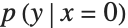
Quiet@Plot[Evaluate@PDF[dist, y], {y, -12, 12}, PlotRange -> All]
ys2 = RandomVariate[distributionAt[#]]& /@ xs;
plot2 = ListPlot[Transpose[{xs, ys2}], PlotStyle -> Opacity[0.4, Hue[0.01, 0.8, 0.8]], PlotRange -> {All, {-12, 12}}]Show[plot, plot2]
likelihoodNet = NetDelete[trainedNet, "neglog"]pairs = CoordinateBoundsArray[{{-12, 12}, {-12, 12}}, .1];
xrange = Flatten[pairs[[All, All, 1]]];
yrange = Flatten[pairs[[All, All, 2]]];nlls = likelihoodNet[<|"x" -> xrange, "y" -> yrange|>];
nlls = Partition[nlls, Length[pairs]];ArrayPlot[Transpose@nlls, Frame -> False, DataReversed -> True,
ColorFunction -> (Opacity[10#, Red]&)]xrange = Range[-12, 12, .1];
{means, stddevs, weights} = Transpose /@ Values[trainedParameterNet[xrange]];Length[xrange]
Dimensions /@ {means, stddevs, weights}colors = Take[ColorData[97, "ColorList"], 6];
plotMixtureComponent[mean_, stddev_, color_] :=
ListLinePlot[{mean - stddev, mean, mean + stddev}, Filling -> {1 -> {2}, 3 -> {2}}, PlotStyle -> {None, color, None}, FillingStyle -> Opacity[0.2, color], PlotRange -> {All, {-12, 12}}]
Show[MapThread[plotMixtureComponent, {means, stddevs, colors}]]StackedListPlot[weights, PlotStyle -> colors]最后,我们尝试同时显示混合分量的平均值和混合权重. 随着混合权重的减少,我们使与该分量相关的线条淡出. 将其与原始数据集进行比较,可以更容易地看到每个 x 值处的主混合分量如何在该 x 值处的原始数据集上反映 y 值的聚类.
plotShadedMean[mean_, weight_, color_] := Module[{winterp = Interpolation[weight]},
	ListLinePlot[mean, ColorFunction -> Function[Lighter[color, 0.9 - winterp[#] * 2]],
	PlotStyle -> Thick, ColorFunctionScaling -> False]]
Show[MapThread[plotShadedMean, {means, weights, colors}], PlotRange -> {All, {-12, 12}}]plot