


DensityPlot
DensityPlot[f,{x,xmin,xmax},{y,ymin,ymax}]
makes a density plot of f as a function of x and y.
DensityPlot[f,{x,y}∈reg]
takes the variables {x,y} to be in the geometric region reg.
Details and Options
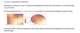
- DensityPlot is also known as heat map.
- It evaluates f at values of x and y in the domain being plotted over and uses a color function
 to map each value f[x,y] to a color.
 - The plot visualizes the set
 where
where  is a color function mapping
  -values to colors.
 - At positions where f does not evaluate to a real number, holes are left so that the background to the density plot shows through.
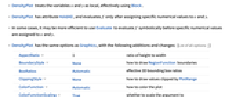
- DensityPlot treats the variables x and y as local, effectively using Block.
- DensityPlot has attribute HoldAll, and evaluates f only after assigning specific numerical values to x and y.
- In some cases, it may be more efficient to use Evaluate to evaluate f symbolically before specific numerical values are assigned to x and y.
- DensityPlot has the same options as Graphics, with the following additions and changes: [List of all options]
-
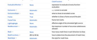
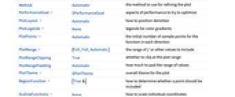
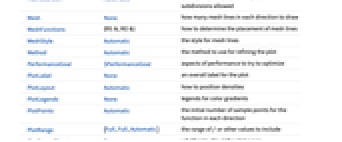
AspectRatio 1 ratio of height to width BoundaryStyle None how to draw RegionFunction boundaries BoxRatios Automatic effective 3D bounding box ratios ClippingStyle None how to draw values clipped by PlotRange ColorFunction Automatic how to color the plot ColorFunctionScaling True whether to scale the argument to ColorFunction EvaluationMonitor None expression to evaluate at every function evaluation Exclusions Automatic x, y curves to exclude ExclusionsStyle None what to draw at excluded curves Frame True whether to draw a frame around the plot FrameTicks Automatic frame tick marks LightingAngle None effective angle of the simulated light source MaxRecursion Automatic the maximum number of recursive subdivisions allowed Mesh None how many mesh lines in each direction to draw MeshFunctions {#1&,#2&} how to determine the placement of mesh lines MeshStyle Automatic the style for mesh lines Method Automatic the method to use for refining the plot PerformanceGoal $PerformanceGoal aspects of performance to try to optimize PlotLayout Automatic how to position densities PlotLegends None legends for color gradients PlotPoints Automatic the initial number of sample points for the function in each direction PlotRange {Full,Full,Automatic} the range of f or other values to include PlotRangeClipping True whether to clip at the plot range PlotRangePadding Automatic how much to pad the range of values PlotTheme $PlotTheme overall theme for the plot RegionFunction (True&) how to determine whether a point should be included ScalingFunctions None how to scale individual coordinates WorkingPrecision MachinePrecision the precision used in internal computations - Typical settings for PlotLegends include:
-
None no legend Automatic automatically determine legend from ColorFunction Placed[lspec,…] specify placement for legend - Possible settings for PlotLayout that show single densities in multiple plot panels include:
-
"Column" use separate densities in a column of panels "Row" use separate densities in a row of panels {"Column",k},{"Row",k} use k columns or rows {"Column",UpTo[k]},{"Row",UpTo[k]} use at most k columns or rows - DensityPlot initially evaluates f at a grid of equally spaced sample points specified by PlotPoints. Then it uses an adaptive algorithm to subdivide at most MaxRecursion times to generate smooth contours.
- You should realize that since it uses only a finite number of sample points, it is possible for DensityPlot to miss features of your functions. To check your results, you should try increasing the settings for PlotPoints and MaxRecursion.
- With the setting Mesh->All, DensityPlot draws mesh lines to show all the subdivisions it uses.
- The default setting MeshFunctions->{#1&,#2&} draws an x, y mesh.
- The arguments supplied to functions in MeshFunctions and RegionFunction are x, y, f.
- ColorFunction is supplied with a single argument, given by default by the scaled value of f.
- With the default settings Exclusions->Automatic and ExclusionsStyle->None, DensityPlot breaks continuity in the density it displays at any discontinuity curve it detects.
- Possible settings for ScalingFunctions include:
-
sf scale the f values {sx,sy} scale x and y axes {sx,sy,sf} scale x and y axes and f values - Each scaling function si is either a string "scale" or {g,g-1} where g-1 is the inverse of g.
- DensityPlot returns Graphics[GraphicsComplex[data]].
-
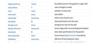
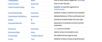
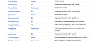
AlignmentPoint Center the default point in the graphic to align with AspectRatio 1 ratio of height to width Axes False whether to draw axes AxesLabel None axes labels AxesOrigin Automatic where axes should cross AxesStyle {} style specifications for the axes Background None background color for the plot BaselinePosition Automatic how to align with a surrounding text baseline BaseStyle {} base style specifications for the graphic BoundaryStyle None how to draw RegionFunction boundaries BoxRatios Automatic effective 3D bounding box ratios ClippingStyle None how to draw values clipped by PlotRange ColorFunction Automatic how to color the plot ColorFunctionScaling True whether to scale the argument to ColorFunction ContentSelectable Automatic whether to allow contents to be selected CoordinatesToolOptions Automatic detailed behavior of the coordinates tool Epilog {} primitives rendered after the main plot EvaluationMonitor None expression to evaluate at every function evaluation Exclusions Automatic x, y curves to exclude ExclusionsStyle None what to draw at excluded curves FormatType TraditionalForm the default format type for text Frame True whether to draw a frame around the plot FrameLabel None frame labels FrameStyle {} style specifications for the frame FrameTicks Automatic frame tick marks FrameTicksStyle {} style specifications for frame ticks GridLines None grid lines to draw GridLinesStyle {} style specifications for grid lines ImageMargins 0. the margins to leave around the graphic ImagePadding All what extra padding to allow for labels etc. ImageSize Automatic the absolute size at which to render the graphic LabelStyle {} style specifications for labels LightingAngle None effective angle of the simulated light source MaxRecursion Automatic the maximum number of recursive subdivisions allowed Mesh None how many mesh lines in each direction to draw MeshFunctions {#1&,#2&} how to determine the placement of mesh lines MeshStyle Automatic the style for mesh lines Method Automatic the method to use for refining the plot PerformanceGoal $PerformanceGoal aspects of performance to try to optimize PlotLabel None an overall label for the plot PlotLayout Automatic how to position densities PlotLegends None legends for color gradients PlotPoints Automatic the initial number of sample points for the function in each direction PlotRange {Full,Full,Automatic} the range of f or other values to include PlotRangeClipping True whether to clip at the plot range PlotRangePadding Automatic how much to pad the range of values PlotRegion Automatic the final display region to be filled PlotTheme $PlotTheme overall theme for the plot PreserveImageOptions Automatic whether to preserve image options when displaying new versions of the same graphic Prolog {} primitives rendered before the main plot RegionFunction (True&) how to determine whether a point should be included RotateLabel True whether to rotate y labels on the frame ScalingFunctions None how to scale individual coordinates Ticks Automatic axes ticks TicksStyle {} style specifications for axes ticks WorkingPrecision MachinePrecision the precision used in internal computations
List of all options


Examples
open all close allBasic Examples (4)
Scope (19)
Sampling (11)
More points are sampled where the function changes quickly:
The plot range is selected automatically:
Areas where the function becomes nonreal are excluded:
The region is split when there are discontinuities in the function:
Use PlotPoints and MaxRecursion to control adaptive sampling:
Use PlotRange to focus in on areas of interest:
Use Exclusions to remove curves or split the resulting surface:
Use RegionFunction to restrict the surface to a region given by inequalities:
The domain may be specified by a region:
The domain may be specified by a MeshRegion:
Presentation (8)
Provide an interactive Tooltip for a surface:
Create a contouring overlay mesh:
Use a theme with simple ticks in a high-contrast color scheme:
Options (89)
AspectRatio (4)
By default, DensityPlot uses the same width and height:
Use a numerical value to specify the height to width ratio:
AspectRatioAutomatic determines the ratio from the plot ranges:
AspectRatioFull adjusts the height and width to tightly fit inside other constructs:
Axes (4)
By default, DensityPlot uses a frame instead of axes:
Use AxesOrigin to specify where the axes intersect:
AxesLabel (4)
No axes labels are drawn by default:
Use labels based on variables specified in DensityPlot:
AxesOrigin (2)
AxesStyle (4)
BoundaryStyle (3)
Use a red boundary around the edges of the surface:
BoundaryStyle applies to regions cut by RegionFunction:
BoundaryStyle does not apply to cuts made by Exclusions:
Use ExclusionsStyle instead:
ClippingStyle (4)
ColorFunction (5)
ColorFunctionScaling (1)
Get the natural range of values by setting ColorFunctionScaling to False:
EvaluationMonitor (2)
Exclusions (6)
ImageSize (7)
Use named sizes such as Tiny, Small, Medium and Large:
Specify the width of the plot:
Specify the height of the plot:
Allow the width and height to be up to a certain size:
Specify the width and height for a graphic, padding with space if necessary:
Setting AspectRatioFull will fill the available space:
Use maximum sizes for the width and height:
Use ImageSizeFull to fill the available space in an object:
Specify the image size as a fraction of the available space:
Mesh (6)
MeshFunctions (3)
MeshStyle (2)
PerformanceGoal (2)
PlotLayout (3)
PlotLegends (4)
Show a legend for the heights:
PlotLegends automatically matches the color function:
Use Placed to change legend position:
Use BarLegend to change legend appearance:
PlotPoints (2)
PlotRange (4)
RegionFunction (3)
ScalingFunctions (9)
By default, plots have linear scales in each direction:
Use a log scale in the ![]() direction:
direction:
Use a linear scale in the ![]() direction that shows smaller numbers at the top:
direction that shows smaller numbers at the top:
Use a reciprocal scale in the ![]() direction:
direction:
Use different scales in the ![]() and
and ![]() directions:
directions:
Reverse the ![]() axis without changing the
axis without changing the ![]() axis:
axis:
Use a scale defined by a function and its inverse:
Positions in Ticks and GridLines are automatically scaled:
PlotRange is automatically scaled:
Applications (7)
Plot a sum of 5 sine waves in random directions:
This shows the solution to the heat equation in one dimension:
Plot a saddle surface; the mesh curves show where the function is zero:
The 1, 2, 3, and ![]() norms, with the iso-norm mesh lines at 1/2, 1, and 3/2:
norms, with the iso-norm mesh lines at 1/2, 1, and 3/2:
Show argument variation for sin, cos, tan, and cot over the complex plane:
Properties & Relations (9)
DensityPlot samples more points where it needs to:
Use ContourPlot to get segmented iso curves and contour regions:
Use ListDensityPlot for plotting continuous data:
Use Plot3D to get 3D surfaces:
Add a ColorFunction to get an overlay density:
ComplexPlot plots the phase of a function using color and shades by the magnitude:
Use ArrayPlot or MatrixPlot for discrete data:
Use Plot for univariate functions:
Use ParametricPlot for plane parametric curves and regions:
Use ContourPlot3D and RegionPlot3D for implicit surfaces and regions:
Possible Issues (2)
With segmenting or piecewise color functions, the transition color borders may not be sharp:
Use ContourPlot for segmenting problems instead:
Color functions or densities that change quickly may show artifacts:
Use PlotPoints to increase the sampling density:
Text
Wolfram Research (1988), DensityPlot, Wolfram Language function, https://reference.wolfram.com/language/ref/DensityPlot.html (updated 2021).
CMS
Wolfram Language. 1988. "DensityPlot." Wolfram Language & System Documentation Center. Wolfram Research. Last Modified 2021. https://reference.wolfram.com/language/ref/DensityPlot.html.
APA
Wolfram Language. (1988). DensityPlot. Wolfram Language & System Documentation Center. Retrieved from https://reference.wolfram.com/language/ref/DensityPlot.html