


VectorDensityPlot
VectorDensityPlot[{{vx,vy},r},{x,xmin,xmax},{y,ymin,ymax}]
generates a vector plot of the vector field {vx,vy} as a function of x and y, superimposed on a density plot of the scalar field r.
VectorDensityPlot[{vx,vy},{x,xmin,xmax},{y,ymin,ymax}]
takes the scalar field to be the norm of the vector field.
VectorDensityPlot[{{vx,vy},{wx,wy},…,r},{x,xmin,xmax},{y,ymin,ymax}]
plots several vector fields.
VectorDensityPlot[…,{x,y}∈reg]
takes the variables {x,y} to be in the geometric region reg.
Details and Options
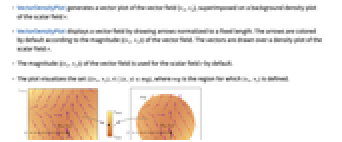
- VectorDensityPlot generates a vector plot of the vector field {vx,vy}, superimposed on a background density plot of the scalar field r.
- VectorDensityPlot displays a vector field by drawing arrows normalized to a fixed length. The arrows are colored by default according to the magnitude
 of the vector field. The vectors are drawn over a density plot of the scalar field r.
 - The magnitude
 of the vector field is used for the scalar field r by default.
 - The plot visualizes the set
 , where
  is the region for which
  is defined.
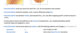
 - VectorDensityPlot omits any vectors for which the vi etc. do not evaluate to real numbers.
- VectorDensityPlot treats the variables x and y as local, effectively using Block.
- VectorDensityPlot has attribute HoldAll, and evaluates the vi, etc. only after assigning specific numerical values to x and y.
- In some cases it may be more efficient to use Evaluate to evaluate the vi, etc. symbolically before specific numerical values are assigned to x and y.
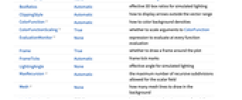
- VectorDensityPlot has the same options as Graphics, with the following additions and changes: [List of all options]
-
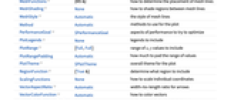
AspectRatio 1 ratio of height to width BoundaryStyle None how to draw RegionFunction boundaries BoxRatios Automatic effective 3D box ratios for simulated lighting ClippingStyle Automatic how to display arrows outside the vector range ColorFunction Automatic how to color background densities ColorFunctionScaling True whether to scale arguments to ColorFunction EvaluationMonitor None expression to evaluate at every function evaluation Frame True whether to draw a frame around the plot FrameTicks Automatic frame tick marks LightingAngle None effective angle for simulated lighting MaxRecursion Automatic the maximum number of recursive subdivisions allowed for the scalar field Mesh None how many mesh lines to draw in the background MeshFunctions {#5&} how to determine the placement of mesh lines MeshShading None how to shade regions between mesh lines MeshStyle Automatic the style of mesh lines Method Automatic methods to use for the plot PerformanceGoal $PerformanceGoal aspects of performance to try to optimize PlotLegends None legends to include PlotRange {Full,Full} range of x, y values to include PlotRangePadding Automatic how much to pad the range of values PlotTheme $PlotTheme overall theme for the plot RegionFunction (True&) determine what region to include ScalingFunctions None how to scale individual coordinates VectorAspectRatio Automatic width-to-length ratio for arrows VectorColorFunction Automatic how to color vectors VectorColorFunctionScaling True whether to scale the arguments to VectorColorFunction VectorMarkers Automatic shape to use for vectors VectorPoints Automatic the number or placement of vectors to plot VectorRange Automatic range of vector lengths to show VectorScaling None how to scale the sizes of arrows VectorSizes Automatic sizes of displayed arrows VectorStyle Automatic how to draw vectors WorkingPrecision MachinePrecision precision to use in internal computations - The arguments supplied to functions in MeshFunctions, RegionFunction, ColorFunction, and VectorColorFunction are x, y, vx, vy, r.
- The default setting MeshFunctions->{#5&} draws mesh lines for the scalar field r.
- Possible settings for ScalingFunctions are:
-
{sx,sy} scale x and y axes - Common built-in scaling functions s include:
-
"Log" 
log scale with automatic tick labeling "Log10" 
base-10 log scale with powers of 10 for ticks "SignedLog" 
log-like scale that includes 0 and negative numbers "Reverse" 
reverse the coordinate direction "Infinite" 
infinite scale -
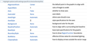
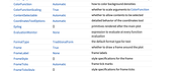
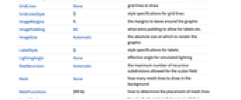
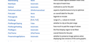
AlignmentPoint Center the default point in the graphic to align with AspectRatio 1 ratio of height to width Axes False whether to draw axes AxesLabel None axes labels AxesOrigin Automatic where axes should cross AxesStyle {} style specifications for the axes Background None background color for the plot BaselinePosition Automatic how to align with a surrounding text baseline BaseStyle {} base style specifications for the graphic BoundaryStyle None how to draw RegionFunction boundaries BoxRatios Automatic effective 3D box ratios for simulated lighting ClippingStyle Automatic how to display arrows outside the vector range ColorFunction Automatic how to color background densities ColorFunctionScaling True whether to scale arguments to ColorFunction ContentSelectable Automatic whether to allow contents to be selected CoordinatesToolOptions Automatic detailed behavior of the coordinates tool Epilog {} primitives rendered after the main plot EvaluationMonitor None expression to evaluate at every function evaluation FormatType TraditionalForm the default format type for text Frame True whether to draw a frame around the plot FrameLabel None frame labels FrameStyle {} style specifications for the frame FrameTicks Automatic frame tick marks FrameTicksStyle {} style specifications for frame ticks GridLines None grid lines to draw GridLinesStyle {} style specifications for grid lines ImageMargins 0. the margins to leave around the graphic ImagePadding All what extra padding to allow for labels etc. ImageSize Automatic the absolute size at which to render the graphic LabelStyle {} style specifications for labels LightingAngle None effective angle for simulated lighting MaxRecursion Automatic the maximum number of recursive subdivisions allowed for the scalar field Mesh None how many mesh lines to draw in the background MeshFunctions {#5&} how to determine the placement of mesh lines MeshShading None how to shade regions between mesh lines MeshStyle Automatic the style of mesh lines Method Automatic methods to use for the plot PerformanceGoal $PerformanceGoal aspects of performance to try to optimize PlotLabel None an overall label for the plot PlotLegends None legends to include PlotRange {Full,Full} range of x, y values to include PlotRangeClipping False whether to clip at the plot range PlotRangePadding Automatic how much to pad the range of values PlotRegion Automatic the final display region to be filled PlotTheme $PlotTheme overall theme for the plot PreserveImageOptions Automatic whether to preserve image options when displaying new versions of the same graphic Prolog {} primitives rendered before the main plot RegionFunction (True&) determine what region to include RotateLabel True whether to rotate y labels on the frame ScalingFunctions None how to scale individual coordinates Ticks Automatic axes ticks TicksStyle {} style specifications for axes ticks VectorAspectRatio Automatic width-to-length ratio for arrows VectorColorFunction Automatic how to color vectors VectorColorFunctionScaling True whether to scale the arguments to VectorColorFunction VectorMarkers Automatic shape to use for vectors VectorPoints Automatic the number or placement of vectors to plot VectorRange Automatic range of vector lengths to show VectorScaling None how to scale the sizes of arrows VectorSizes Automatic sizes of displayed arrows VectorStyle Automatic how to draw vectors WorkingPrecision MachinePrecision precision to use in internal computations
List of all options


Examples
open all close allBasic Examples (4)
Scope (19)
Sampling (9)
Visualize a vector field with the background based on ![]() :
:
Use Evaluate to evaluate the vector field symbolically before numeric assignment:
Plot a vector field with vectors placed with specified densities:
Plot the vectors that go through a set of seed points:
Create a hexagonal grid of field vectors with a different number of arrows for ![]() and
and ![]() :
:
Specify a list of points for showing field vectors:
Plot vectors over a specified region:
The domain may be specified by a region:
The domain may be specified by a MeshRegion:
Presentation (10)
Plot a vector field with arrows scaled according to their magnitudes:
Use a single color for the arrows:
Specify the sizes of the arrows:
Plot a vector field with the background and vectors colored according to the field magnitude:
Use a named appearance to draw the vectors:
VectorColorFunction takes precedence over colors in VectorStyle:
Set VectorColorFunctionNone to specify colors with VectorStyle:
Set the marker style for multiple vector fields:
Include a legend for the scalar field:
Options (84)
ColorFunction (5)
Color the scalar field magnitude with a named color gradient from ColorData:
Specify a different scalar field:
Use ColorData for predefined color gradients:
Specify a color function that blends two colors by the ![]() coordinate:
coordinate:
Use ColorFunctionScaling->False to get unscaled values:
ColorFunctionScaling (4)
By default, scaled values are used:
Use ColorFunctionScaling->False to get unscaled values:
Use unscaled coordinates in the ![]() direction and scaled coordinates in the
direction and scaled coordinates in the ![]() direction:
direction:
Explicitly specify the scaling for each color function argument:
EvaluationMonitor (2)
Mesh (5)
MeshFunctions (3)
MeshShading (3)
PerformanceGoal (2)
PlotRange (3)
RegionBoundaryStyle (6)
Show the region being plotted:
Show the region defined by a region function:
The boundaries of full rectangular regions are not shown:
Use None to not show the boundary:
RegionFunction (3)
VectorAspectRatio (2)
VectorColorFunction (5)
Color the vectors according to their norm:
Color the vectors according to a different scalar field:
Use any named color gradient from ColorData:
Color the vectors according to their ![]() values:
values:
Use VectorColorFunctionScaling->False to get unscaled values:
VectorColorFunctionScaling (4)
By default, scaled values are used:
Use VectorColorFunctionScaling->False to get unscaled values:
Use unscaled coordinates in the ![]() direction and scaled coordinates in the
direction and scaled coordinates in the ![]() direction:
direction:
Explicitly specify the scaling for each color function argument:
VectorMarkers (4)
VectorPoints (9)
Use automatically determined vector points:
Use symbolic names to specify the set of field vectors:
Create a hexagonal grid of field vectors with the same number of arrows for ![]() and
and ![]() :
:
Create a hexagonal grid of field vectors with a different number of arrows for ![]() and
and ![]() :
:
Specify a list of points for showing field vectors:
Use a different number of field vectors on a hexagonal grid:
The location for vectors is given in the middle of the drawn vector:
Use a rectangular mesh instead of a hexagonal mesh:
Use a mesh generated from a triangularization of the region:
VectorRange (4)
VectorScaling (2)
VectorSizes (3)
VectorStyle (6)
VectorColorFunction takes precedence over colors in VectorStyle:
Set VectorColorFunctionNone to specify colors with VectorStyle:
Set the style for multiple vector fields:
Plot the vector fields without arrowheads:
Use Arrowheads to specify an explicit style of the arrowheads:
Specify both arrow tail and head:
Graphics primitives without Arrowheads are scaled:
Applications (3)
Properties & Relations (10)
Use ListStreamDensityPlot to plot streamlines instead of vectors:
Use ListVectorDensityPlot or ListStreamDensityPlot to plot with data:
Use VectorPlot to plot functions without a density plot:
Use StreamPlot to plot with streamlines instead of vectors:
Use ListVectorPlot or ListStreamPlot to plot with data:
Use LineIntegralConvolutionPlot to plot the line integral convolution of a vector field:
Use VectorDisplacementPlot to visualize the deformation of a region associated with a displacement vector field:
Use ListVectorDisplacementPlot to visualize the same deformation based on data:
Use VectorPlot3D or StreamPlot3D to visualize 3D vector fields:
Use ListVectorPlot3D or ListStreamPlot3D to plot with data:
Use SliceVectorPlot3D to visualize 3D vector fields along a surface:
Use ListSliceVectorPlot3D to plot with data:
Use VectorDisplacementPlot3D to visualize the deformation of a 3D region associated with a displacement vector field:
Use ListVectorDisplacementPlot3D to visualize the same deformation based on data:
Scalar fields can be plotted by themselves with DensityPlot:
Use ComplexVectorPlot or ComplexStreamPlot to visualize a complex function of a complex variable as a vector field or with streamlines:
Use GeoVectorPlot to plot vectors on a map:
Use GeoStreamPlot to plot streamlines instead of vectors:
Text
Wolfram Research (2008), VectorDensityPlot, Wolfram Language function, https://reference.wolfram.com/language/ref/VectorDensityPlot.html (updated 2022).
CMS
Wolfram Language. 2008. "VectorDensityPlot." Wolfram Language & System Documentation Center. Wolfram Research. Last Modified 2022. https://reference.wolfram.com/language/ref/VectorDensityPlot.html.
APA
Wolfram Language. (2008). VectorDensityPlot. Wolfram Language & System Documentation Center. Retrieved from https://reference.wolfram.com/language/ref/VectorDensityPlot.html