


ListStreamPlot
ListStreamPlot[varr]
generates a stream plot from an array varr of vectors.
ListStreamPlot[{{{x1,y1},{vx1,vy1}},…}]
generates a stream plot from vectors {vxi,vyi} given at points {xi,yi}.
ListStreamPlot[{data1,data2,…}]
plots data for several vector fields.
Details and Options
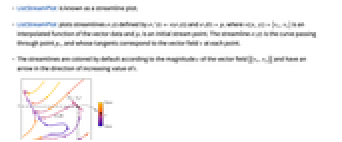
- ListStreamPlot is known as a streamline plot.
- ListStreamPlot plots streamlines
 defined by
  and
and  where
where  is an interpolated function of the vector data and
  is an initial stream point. The streamline
  is the curve passing through point
  , and whose tangents correspond to the vector field
  at each point.
 - The streamlines are colored by default according to the magnitude
 of the vector field
  and have an arrow in the direction of increasing value of
  .
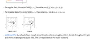
. - For regular data, the vector field
 has value varr〚i,j〛 at
  .
. - For irregular data, the vector field
 has value {vxi,vyi} at
  .
. - ListStreamPlot by default shows enough streamlines to achieve a roughly uniform density throughout the plot and shows no background scalar field. This is independent of the vector locations.
- ListStreamPlot by default interpolates the data given and shows enough streamlines to achieve a roughly uniform density throughout the plot.
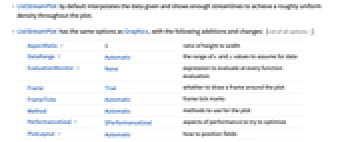
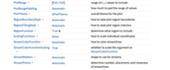
- ListStreamPlot has the same options as Graphics, with the following additions and changes: [List of all options]
-
AspectRatio 1 ratio of height to width DataRange Automatic the range of x and y values to assume for data EvaluationMonitor None expression to evaluate at every function evaluation Frame True whether to draw a frame around the plot FrameTicks Automatic frame tick marks Method Automatic methods to use for the plot PerformanceGoal $PerformanceGoal aspects of performance to try to optimize PlotLayout Automatic how to position fields PlotRange {Full,Full} range of x, y values to include PlotRangePadding Automatic how much to pad the range of values PlotTheme $PlotTheme overall theme for the plot RegionBoundaryStyle Automatic how to style plot region boundaries RegionFillingStyle Automatic how to style plot region interiors RegionFunction True& determine what region to include ScalingFunctions None how to scale individual coordinates StreamColorFunction Automatic how to color streamlines StreamColorFunctionScaling True whether to scale the argument to StreamColorFunction StreamMarkers Automatic shape to use for streams StreamPoints Automatic determine number, placement, and closeness of streamlines StreamScale Automatic determine sizes and segmenting of individual streamlines StreamStyle Automatic how to draw streamlines WorkingPrecision MachinePrecision precision to use in internal computations - The arguments supplied to functions in RegionFunction and StreamColorFunction are x, y, vx, vy, Norm[{vx,vy}].
- Possible settings for PlotLayout that show single streamlines in multiple plot panels include:
-
"Column" use separate streamlines in a column of panels "Row" use separate streamlines in a row of panels {"Column",k},{"Row",k} use k columns or rows {"Column",UpTo[k]},{"Row",UpTo[k]} use at most k columns or rows - Possible settings for ScalingFunctions are:
-
{sx,sy} scale x and y axes - Common built-in scaling functions s include:
-
"Log" 
log scale with automatic tick labeling "Log10" 
base-10 log scale with powers of 10 for ticks "SignedLog" 
log-like scale that includes 0 and negative numbers "Reverse" 
reverse the coordinate direction "Infinite" 
infinite scale -
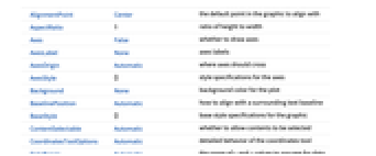
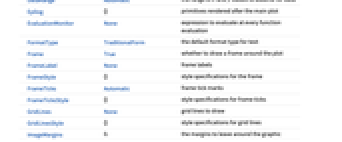
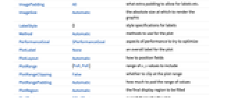
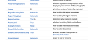
AlignmentPoint Center the default point in the graphic to align with AspectRatio 1 ratio of height to width Axes False whether to draw axes AxesLabel None axes labels AxesOrigin Automatic where axes should cross AxesStyle {} style specifications for the axes Background None background color for the plot BaselinePosition Automatic how to align with a surrounding text baseline BaseStyle {} base style specifications for the graphic ContentSelectable Automatic whether to allow contents to be selected CoordinatesToolOptions Automatic detailed behavior of the coordinates tool DataRange Automatic the range of x and y values to assume for data Epilog {} primitives rendered after the main plot EvaluationMonitor None expression to evaluate at every function evaluation FormatType TraditionalForm the default format type for text Frame True whether to draw a frame around the plot FrameLabel None frame labels FrameStyle {} style specifications for the frame FrameTicks Automatic frame tick marks FrameTicksStyle {} style specifications for frame ticks GridLines None grid lines to draw GridLinesStyle {} style specifications for grid lines ImageMargins 0. the margins to leave around the graphic ImagePadding All what extra padding to allow for labels etc. ImageSize Automatic the absolute size at which to render the graphic LabelStyle {} style specifications for labels Method Automatic methods to use for the plot PerformanceGoal $PerformanceGoal aspects of performance to try to optimize PlotLabel None an overall label for the plot PlotLayout Automatic how to position fields PlotRange {Full,Full} range of x, y values to include PlotRangeClipping False whether to clip at the plot range PlotRangePadding Automatic how much to pad the range of values PlotRegion Automatic the final display region to be filled PlotTheme $PlotTheme overall theme for the plot PreserveImageOptions Automatic whether to preserve image options when displaying new versions of the same graphic Prolog {} primitives rendered before the main plot RegionBoundaryStyle Automatic how to style plot region boundaries RegionFillingStyle Automatic how to style plot region interiors RegionFunction True& determine what region to include RotateLabel True whether to rotate y labels on the frame ScalingFunctions None how to scale individual coordinates StreamColorFunction Automatic how to color streamlines StreamColorFunctionScaling True whether to scale the argument to StreamColorFunction StreamMarkers Automatic shape to use for streams StreamPoints Automatic determine number, placement, and closeness of streamlines StreamScale Automatic determine sizes and segmenting of individual streamlines StreamStyle Automatic how to draw streamlines Ticks Automatic axes ticks TicksStyle {} style specifications for axes ticks WorkingPrecision MachinePrecision precision to use in internal computations
List of all options


Examples
open all close allBasic Examples (3)
Scope (22)
Sampling (9)
Plot streamlines for a regular collection of vectors, and give a data range for the domain:
Plot streamlines for an irregular collection of vectors:
Plot streamlines for several vector fields:
Plot a vector field with streamlines placed with specified densities:
Plot the streamlines that go through a set of seed points:
Use both automatic and explicit seeding with styles for explicitly seeded streamlines:
Plot streamlines over a specified region:
Presentation (13)
Specify different dashings and arrowheads by settings to StreamScale:
Streamlines with arrows are colored by default according to the magnitude of the field:
Use a constant color for the streamlines:
Show multiple vector fields in separate panels:
Use a column instead of a row:
Style streamlines for multiple vector fields:
Use a named appearance to draw the streamlines:
Style the streamlines as well:
Specify mesh lines with different styles:
Specify global mesh line styles:
Shade mesh regions cyclically:
Apply a variety of styles to region boundaries:
Use a theme with simple ticks and grid lines:
Options (98)
AspectRatio (3)
By default, ListStreamPlot uses the same width and height:
Use a numerical value to specify the height to width ratio:
AspectRatioAutomatic determines the ratio from the plot ranges:
Axes (4)
By default, ListStreamPlot uses a frame instead of axes:
Use AxesOrigin to specify where the axes intersect:
AxesStyle (4)
DataRange (1)
ImageSize (5)
Use named sizes such as Tiny, Small, Medium, and Large:
Specify the width of the plot:
Specify the height of the plot:
Allow the width and height to be up to a certain size:
Specify the width and height for a graphic, padding with space if necessary:
Setting AspectRatioFull will fill the available space:
Mesh (5)
MeshFunctions (3)
MeshShading (3)
PerformanceGoal (2)
PlotLayout (3)
PlotLegends (5)
Use legends for multiple datasets:
Use SwatchLegend to add an overall legend label:
Legends automatically pick up styles and shapes:
Use a legend for the color function:
Use Placed to put legends above the plot:
PlotRange (7)
RegionBoundaryStyle (3)
RegionFillingStyle (3)
RegionFunction (3)
ScalingFunctions (3)
StreamColorFunction (5)
By default, color streamlines according to the norm of the vector field:
Use any named color gradient from ColorData:
Use ColorData for predefined color gradients:
Specify a color function that blends two colors by the ![]() coordinate:
coordinate:
Use StreamColorFunctionScaling->False to get unscaled values:
StreamColorFunctionScaling (4)
By default, scaled values are used:
Use StreamColorFunctionScaling->False to get unscaled values:
Use unscaled coordinates in the ![]() direction and scaled coordinates in the
direction and scaled coordinates in the ![]() direction:
direction:
Explicitly specify the scaling for each color function argument:
StreamMarkers (8)
StreamPoints (6)
Specify a maximum number of streamlines:
Use symbolic names to specify the number of streamlines:
Use both automatic and explicit seeding with styles for explicitly seeded streamlines:
Specify the minimum distance between streamlines:
Specify the minimum distance between streamlines at the start and end of a streamline:
StreamScale (9)
Create full streamlines without segmentation:
Use symbolic names to control the lengths of streamlines:
Specify an explicit dashing pattern for streamlines:
Specify number of points rendered on each streamline segment:
Specify absolute aspect ratios relative to the longest line segment:
Specify relative aspect ratios relative to each line segment:
StreamStyle (5)
StreamColorFunction has precedence over colors specified in StreamStyle:
Set StreamColorFunctionNone to specify colors with StreamStyle:
Applications (6)
Global attractor of damped conservative system:
Visualize the first horizontal and vertical Gaussian derivatives of an image:
Combine the vertical and horizontal Gaussian derivatives:
Compute wind velocity from given coordinates:
Organize several datasets into a tabbed view:
Explore various streamline styles and scales with several examples:
Generate icons to graphically represent field choices:
Click on the field icons to switch field plots:
Consider the heat equation ![]() on the unit square with
on the unit square with ![]() on the left edge,
on the left edge, ![]() (insulated) on the top and bottom edges, and
(insulated) on the top and bottom edges, and ![]() for
for ![]() and
and ![]() for
for ![]() on the right edge.
on the right edge.
Use finite differences to discretize the equation and the boundary conditions:
Solve the equations and compute the temperature gradients:
Plot the approximate temperatures with ListContourPlot and the heat flux with ListStreamPlot:
Properties & Relations (10)
Use StreamPlot for plotting functions:
Use ListVectorPlot for plotting data without a density plot of the scalar field:
Use ListStreamDensityPlot for plotting data with a density plot of the scalar field:
Use ListVectorDensityPlot to plot arrows instead of streams:
Use StreamDensityPlot to plot functions with a density plot of the scalar field:
Use VectorPlot to plot functions with vectors instead of streamlines:
Use ListVectorDisplacementPlot to visualize the deformation of a region associated with a displacement vector field:
Use ListVectorDisplacementPlot3D to visualize a deformation in 3D:
Use ListLineIntegralConvolutionPlot to plot the line integral convolution of vector field data:
Use ListVectorPlot3D and ListStreamPlot3D to visualize 3D vector field data:
Use ListSliceVectorPlot3D to plot a 3D vector field on a specified surface:
Use GeoStreamPlot to plot streams on a map:
Use GeoVectorPlot to plot arrows instead of streams:
Text
Wolfram Research (2008), ListStreamPlot, Wolfram Language function, https://reference.wolfram.com/language/ref/ListStreamPlot.html (updated 2022).
CMS
Wolfram Language. 2008. "ListStreamPlot." Wolfram Language & System Documentation Center. Wolfram Research. Last Modified 2022. https://reference.wolfram.com/language/ref/ListStreamPlot.html.
APA
Wolfram Language. (2008). ListStreamPlot. Wolfram Language & System Documentation Center. Retrieved from https://reference.wolfram.com/language/ref/ListStreamPlot.html