


DiscretePlot
DiscretePlot[f,{n,nmax}]
generates a plot of f as a function of n when n=1,…,nmax.
DiscretePlot[f,{n,nmin,nmax}]
generates a plot when n runs from nmin to nmax.
DiscretePlot[f,{n,nmin,nmax,dn}]
uses steps dn.
DiscretePlot[f,{n,{n1,…,nm}}]
uses the successive values n1, …, nm.
DiscretePlot[{f1,f2,…},…]
plots the values of all the fi.
Details and Options
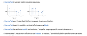

- DiscretePlot is typically used to visualize sequences.
- DiscretePlot uses the standard Wolfram Language iterator specification.
- DiscretePlot treats the variable n as local, effectively using Block.
- DiscretePlot has attribute HoldAll and evaluates f only after assigning specific numerical values to n.
- In some cases, it may be more efficient to use Evaluate to evaluate f symbolically before specific numerical values are assigned to n.
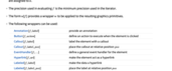
- The precision used in evaluating f is the minimum precision used in the iterator.
- The form w[f] provides a wrapper w to be applied to the resulting graphics primitives.
- The following wrappers can be used:
-
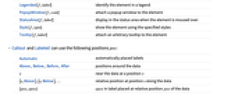
Annotation[f,label] provide an annotation Button[f,action] define an action to execute when the element is clicked Callout[f,label] label the element with a callout Callout[f,label,pos] place the callout at relative position pos EventHandler[f,…] define a general event handler for the element Hyperlink[f,uri] make the element act as a hyperlink Labeled[f,label] make the data a hyperlink Labeled[f,label,pos] place the label at relative position pos Legended[f,label] identify the element in a legend PopupWindow[f,cont] attach a popup window to the element StatusArea[f,label] display in the status area when the element is moused over Style[f,opts] show the element using the specified styles Tooltip[f,label] attach an arbitrary tooltip to the element - Callout and Labeled can use the following positions pos:
-
Automatic automatically placed labels Above, Below, Before, After positions around the data x near the data at a position x {s,Above},{s,Below},… relative position at position s along the data {pos,epos} epos in label placed at relative position pos of the data - Labels that depend on n will be applied for each plot element, while labels that are independent of n will only occur once.
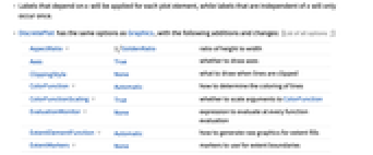
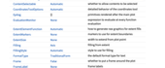
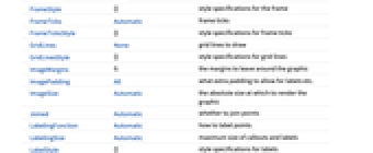
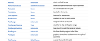
- DiscretePlot has the same options as Graphics, with the following additions and changes: [List of all options]
-
AspectRatio 1/GoldenRatio ratio of height to width Axes True whether to draw axes ClippingStyle None what to draw when lines are clipped ColorFunction Automatic how to determine the coloring of lines ColorFunctionScaling True whether to scale arguments to ColorFunction EvaluationMonitor None expression to evaluate at every function evaluation ExtentElementFunction Automatic how to generate raw graphics for extent fills ExtentMarkers None markers to use for extent boundaries ExtentSize None width to extend from plot point Filling Axis filling from extent FillingStyle Automatic style to use for filling Joined Automatic whether to join points LabelingFunction Automatic how to label points LabelingSize Automatic maximum size of callouts and labels Method Automatic what method to use PerformanceGoal $PerformanceGoal aspects of performance to try to optimize PlotLabels None labels for elements PlotLegends None legends for sequences PlotMarkers None markers to use for plot points PlotRange Automatic range of values to include PlotRangeClipping True whether to clip at the plot range PlotStyle Automatic graphics directives to determine the style of each line PlotTheme $PlotTheme overall theme for the plot RegionFunction (True &) how to determine whether a point should be included ScalingFunctions None how to scale individual coordinates WorkingPrecision MachinePrecision precision for internal computation - The arguments supplied to ColorFunction are
 ,
,  .
. - With the setting ExtentSize->{sl,sr}, a horizontal line is drawn around each plot point, extending sl to the left and sr to the right. With ExtentMarkers->{ml,mr}, the markers ml and mr will be used as left and right extent boundary markers.
- With the default settings Joined->Automatic and Filling->Axis, DiscretePlot switches between drawing points with a stem filling when there are few points and lines with a solid filling when there are many points.
- The arguments supplied to ExtentElementFunction are the element region {{xmin,xmax},{ymin,ymax}} and the sample point {xi,yi}.
- With the setting ExtentSize->None, xmin is equal to xmax. With the setting Filling->None, ymin is equal to ymax.
- ColorData["DefaultPlotColors"] gives the default sequence of colors used by PlotStyle.
- Possible settings for ScalingFunctions include:
-
sy scale the y axis {sx,sy} scale x and y axes - Each scaling function si is either a string "scale" or {g,g-1}, where g-1 is the inverse of g.
-
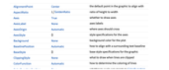
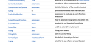
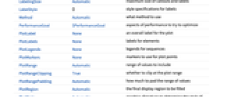
AlignmentPoint Center the default point in the graphic to align with AspectRatio 1/GoldenRatio ratio of height to width Axes True whether to draw axes AxesLabel None axes labels AxesOrigin Automatic where axes should cross AxesStyle {} style specifications for the axes Background None background color for the plot BaselinePosition Automatic how to align with a surrounding text baseline BaseStyle {} base style specifications for the graphic ClippingStyle None what to draw when lines are clipped ColorFunction Automatic how to determine the coloring of lines ColorFunctionScaling True whether to scale arguments to ColorFunction ContentSelectable Automatic whether to allow contents to be selected CoordinatesToolOptions Automatic detailed behavior of the coordinates tool Epilog {} primitives rendered after the main plot EvaluationMonitor None expression to evaluate at every function evaluation ExtentElementFunction Automatic how to generate raw graphics for extent fills ExtentMarkers None markers to use for extent boundaries ExtentSize None width to extend from plot point Filling Axis filling from extent FillingStyle Automatic style to use for filling FormatType TraditionalForm the default format type for text Frame False whether to put a frame around the plot FrameLabel None frame labels FrameStyle {} style specifications for the frame FrameTicks Automatic frame ticks FrameTicksStyle {} style specifications for frame ticks GridLines None grid lines to draw GridLinesStyle {} style specifications for grid lines ImageMargins 0. the margins to leave around the graphic ImagePadding All what extra padding to allow for labels etc. ImageSize Automatic the absolute size at which to render the graphic Joined Automatic whether to join points LabelingFunction Automatic how to label points LabelingSize Automatic maximum size of callouts and labels LabelStyle {} style specifications for labels Method Automatic what method to use PerformanceGoal $PerformanceGoal aspects of performance to try to optimize PlotLabel None an overall label for the plot PlotLabels None labels for elements PlotLegends None legends for sequences PlotMarkers None markers to use for plot points PlotRange Automatic range of values to include PlotRangeClipping True whether to clip at the plot range PlotRangePadding Automatic how much to pad the range of values PlotRegion Automatic the final display region to be filled PlotStyle Automatic graphics directives to determine the style of each line PlotTheme $PlotTheme overall theme for the plot PreserveImageOptions Automatic whether to preserve image options when displaying new versions of the same graphic Prolog {} primitives rendered before the main plot RegionFunction (True &) how to determine whether a point should be included RotateLabel True whether to rotate y labels on the frame ScalingFunctions None how to scale individual coordinates Ticks Automatic axes ticks TicksStyle {} style specifications for axes ticks WorkingPrecision MachinePrecision precision for internal computation
List of all options
Examples
open all close allBasic Examples (4)
Scope (19)
Data and Wrappers (4)
Use wrappers on functions or sets of functions:
Override the default tooltips:
Use PopupWindow to provide additional drilldown information:
Button can be used to trigger any action:
Use ScalingFunctions to scale the axes:
Labeling and Legending (8)
Apply callouts to extended regions:
Use Legended to provide a legend for a specific dataset:
Use Placed to change the legend location:
Use Callout to label datasets:
Use Callout to label elements:
Use Callout to label elements even when they are joined:
Specify a location for labels:
Specify label names with LabelingFunction:
Styling and Appearance (7)
Use an explicit list of styles for the plots:
Style can be used to override styles:
Use any graphic for PlotMarkers:
Use any gradient or indexed color schemes from ColorData:
Use ExtentSize to associate a region with a point:
Options (80)
AspectRatio (4)
By default, DiscretePlot uses a fixed height to width ratio for the plot:
Make the height the same as the width with AspectRatio1:
AspectRatioAutomatic determines the ratio from the plot ranges:
AspectRatioFull adjusts the height and width to tightly fit inside other constructs:
ColorFunction (6)
Color by scaled ![]() and
and ![]() coordinates, respectively:
coordinates, respectively:
Color filling element functions:
Color by height with a named color scheme:
ColorFunction has higher priority than PlotStyle:
ColorFunctionScaling (2)
ExtentElementFunction (5)
Get a list of built-in settings for ExtentElementFunction:
For detailed settings, use Palettes ▶ Chart Element Schemes:
This ChartElementFunction is appropriate to show the global scale:
Write a custom ExtentElementFunction:
Built-in element functions may have options; use Palettes ▶ Chart Element Schemes to set them:
ExtentMarkers (6)
Do not show the extent endpoints:
Use points to show the extent endpoints:
Show ![]() with appropriate continuity markers:
with appropriate continuity markers:
Show ![]() with appropriate continuity markers:
with appropriate continuity markers:
Use custom shapes for the markers:
Markers use the settings for PlotStyle:
ExtentSize (6)
Filling (6)
DiscretePlot automatically fills to the axis:
Use symbolic or explicit values:
With ExtentSize->Full:
Fill between curves 1 and 2 with a specific style:
Fill between curves 1 and 2; use red when 1 is below 2 and blue when 1 is above 2:
FillingStyle (4)
Fill with red below the ![]() axis and blue above:
axis and blue above:
Use a variable filling style obtained from a ColorFunction:
Joined (3)
LabelingFunction (3)
PlotLabels (4)
Specify text to label sets of points:
Place the labels above the points:
Use callouts to identify the points:
Use None to not add a label:
PlotLegends (6)
Generate a legend using labels:
Generate a legend using placeholders:
Use PlotLegends->"Expressions" to use the actual equations:
PlotLegends matches PlotStyle and PlotMarkers in the plot:
Use Placed to change legend position:
Use PointLegend to change legend appearance:
PlotMarkers (8)
DiscretePlot normally uses distinct colors to distinguish different sets of data:
Automatically use colors and shapes to distinguish sets of data:
Markers are placed at the plot points regardless of the setting for ExtentSize:
Change the size of the default plot markers:
Use arbitrary text for plot markers:
Use explicit graphics for plot markers:
PlotStyle (4)
Use different style directives:
By default, different styles are chosen for multiple curves and regions:
Explicitly specify the style for different curves and regions:
PlotStyle can be combined with ColorFunction:
ScalingFunctions (7)
By default, plots have linear scales in each direction:
Use a linear scale in the ![]() direction that shows smaller numbers at the top:
direction that shows smaller numbers at the top:
Use a log scale in the ![]() direction:
direction:
Reverse the ![]() axis without changing the
axis without changing the ![]() axis:
axis:
Use different scales in the ![]() and
and ![]() directions:
directions:
Use a scale defined by a function and its inverse:
PlotRange and AxesOrigin are automatically scaled:
Applications (4)
Properties & Relations (4)
Plot generates continuous curves:
Use ListPlot to plot lists of values:
Use BarChart to show bars for lists of values:
Use DiscretePlot3D to plot functions of two discrete variables:
Text
Wolfram Research (2008), DiscretePlot, Wolfram Language function, https://reference.wolfram.com/language/ref/DiscretePlot.html (updated 2019).
CMS
Wolfram Language. 2008. "DiscretePlot." Wolfram Language & System Documentation Center. Wolfram Research. Last Modified 2019. https://reference.wolfram.com/language/ref/DiscretePlot.html.
APA
Wolfram Language. (2008). DiscretePlot. Wolfram Language & System Documentation Center. Retrieved from https://reference.wolfram.com/language/ref/DiscretePlot.html