|
2. Kinematic Modeling OverviewThis chapter covers the building and running of basic kinematic models with MechanicalSystems. Throughout this chapter the simplest and most commonly used forms of each MechanicalSystems command are presented. For more detailed information on specific commands, consult the reference guide in the appendix.
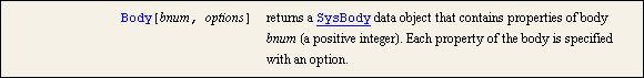
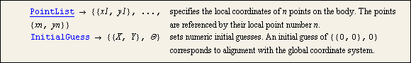
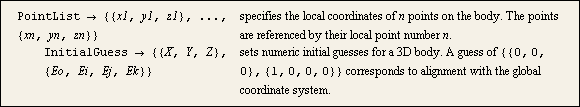
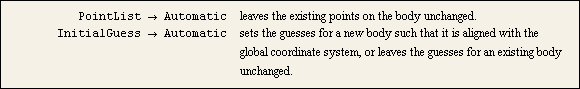
MechanicalSystems follows most of the conventions set by Mathematica as to its use of function names, options, and option settings. One significant deviation from standard Mathematica practice is that MechanicalSystems often uses the same name for an option and for the name of a function that performs a service related to the option. For example, PointList is the name of an option that is used to set the values of local point coordinates, and it is also the name of a function that queries the local point coordinates. 2.1 Body ObjectsA SysBody object is a Mech data object that is used to define the points and properties of a mechanism body. It is not necessary to use body objects in Mech kinematic models, as demonstrated in Sections 1.2 and 1.3, but the use of body objects allows points to be defined once, inside the body object, and then to be referenced throughout the Mech model. This can reduce the likelihood of error due to changing the definition of a point at one place on the model, while failing to change it elsewhere. 2.1.1 BodyMech SysBody objects are created by the Body function, and used to define specific properties of a body in a mechanism model. A function to define body objects. Body accepts three options for defining inertia properties of a body: Mass, Inertia, and Centroid. These options will be discussed further in Section 8.1. The options for Body that are relevant in the kinematic phase of analysis are the PointList and InitialGuess options. 2D2D options for Body. 3D3D options for Body. 2D/3DDefault option settings for Body. Executing the Body function does not, in itself, have any affect on the current Mech model. The returned body objects must be added to the model with the SetBodies command, which is discussed in Section 2.1.2.
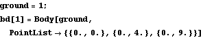
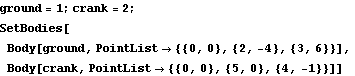
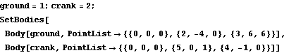
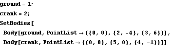
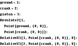
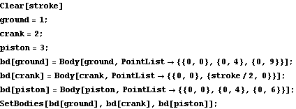
Initial guesses specified with a body object are referred to as the permanent initial guesses. These initial guesses are used the first time that a solution is sought with SolveMech. Each subsequent solution attempt uses the previous solution as its initial guess. When the initial guesses are set with SetGuess, they may be explicitly set to user-specified values, or reset to the stored values of the permanent initial guesses. ExampleThis loads the Modeler2D package. The 2D example mechanism of Section 1.2 can be modified to use three body objects instead of repeatedly calling out the several local point coordinates on the ground, crankshaft, and piston bodies. These body objects store the local point definitions for future reference, through their integer point numbers, by other Mech functions. Here are the crankshaft-piston mechanism bodies.
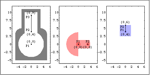
The ground body object uses three local point definitions.
P1 is a point at the global origin that is the rotational axis of the crankshaft.
P2 and P3 are two points that define the vertical line upon which the piston translates.This defines a body object for the ground body.
Out[3]= |  |
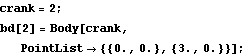
The crankshaft uses two local point definitions.
P1 is a point at the local origin that is the rotational axis of the crankshaft.
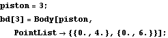
P2 is a point on the local x axis that is the attachment point of the connecting rod.This defines a body object for the piston. The piston also uses two local point definitions.
P1 is a point on the local y axis that is the attachment point of the connecting rod.
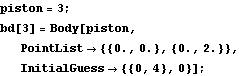
P2 is a point on the local y axis that is the upper end of the translation line of the piston. This defines a body object for the piston. InitialGuessAlternately, the piston could have been defined with the local origin at the attachment point of the connecting rod. This would suggest that a different initial guess be used than the default of X3 = 0, Y3 = 0,  3 = 0. 3 = 0. Here is a body object for the piston with relocated origin and corresponding initial guess. This body object functions identically to the first one, except the Y coordinate of the piston is always 4 units greater, because the origin of the body has moved 4 units upward.
Note that each of these body objects must be added to the current model with SetBodies before they will have any effect on the model. 2.1.2 SetBodiesThe Mech SetBodies function is used to apply the data contained in body objects to the current kinematic model. The body object processing function. All properties specified in a call to SetBodies overwrite properties that are currently defined unless the property specification is the default, Automatic, in which case the property is left unchanged.
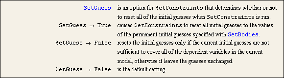
If SetBodies is passed a body object with an InitialGuess specification other than Automatic, the current initial guesses of each body are reset to the values of the permanent initial guesses.
There is a subtle issue regarding the use of the PointList specification with SetBodies. When SetBodies is run with a new InitialGuess specification, the changed guess is immediately reflected in Mech's internal database. The same holds true for changing inertia properties with SetBodies; the mass matrix is immediately updated.
However, changing the coordinates of a point with PointList must reflect a change throughout the constraint equations defined with SetConstraints. This cannot be done without rebuilding the constraint equations. Therefore, if the constraint equations have already been built with SetConstraints when SetBodies is passed a PointList specification other than Automatic, the constraint equations will all be automatically rebuilt by SetConstraints the next time that a solution is sought, which may cause a noticeable delay in the operation of SolveMech.
The following command incorporates the three body objects that were defined in Section 2.1.1 into the current model. This starts a model with the three body objects. SetBodies returns Null. All of the mechanism points and properties passed to SetBodies are stored in Mech's internal database.
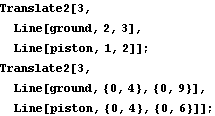
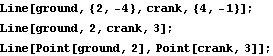
Now that local point definitions have been added to the current model, they can be referenced by their local point numbers in any Mech function. Instead of using the local coordinates of a point, simply use the integer point number. For example, the Translate2 constraint in the crankshaft-piston model would use four local point numbers instead of the four explicit 2D coordinates in the Line objects. Here is a constraint with, and without, local point numbers. Updating PropertiesSetBodies only sets the values of the properties that are not specified with the default, Automatic. Thus, SetBodies can be used to update the value of individual body properties without affecting properties already defined. This updates only the crankshaft's initial guess. PointListNote that PointList, like many Mech options, can also be used as a function. Another usage of PointList. Here are the local coordinates of point 2 on the piston.
Out[14]= |  |
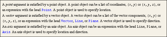
2.2 Points, Vectors, and AxesThis section explains the functionality and syntax of Mech's method of defining the basic geometric entities that make up a mechanism model: points, vectors, and axes. A look at the usage statements for most of Mech's functions shows that they take arguments of type point, vector, or axis. In all cases there are several ways to specify a point, vector, or axis, depending on whether the entity is defined in global or local coordinates, is located entirely on a single body, or spans across multiple bodies. The three basic types of Mech geometry objects. 2.2.1 PointsThe most basic geometric entity used by Mech is the point object. Point objects reference the location of a 2D or 3D point in global coordinates or in local coordinates on a specified body. Point objects may be given as 2D or 3D vectors, or they may have the head Point just like the built-in Mathematica graphics primitive. This does not lead to any conflict or require a redefinition of Point because it has no definition by default. The Point head is only used to hold its arguments in Mech, just as it is in standard Mathematica.
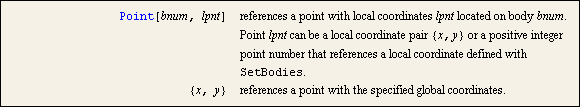
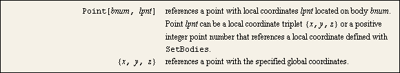
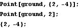
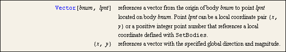
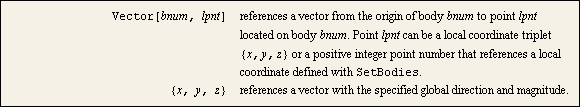
Any Mech function that calls for a point object accepts either of the following syntax. 2DMethods of defining 2D point objects. 3DMethods of defining 3D point objects. Assuming that the appropriate body object definition has been made, any point on any body can be referenced through either its global coordinates, its local coordinates, or its local coordinate number. The following example shows several point objects that are functionally identical. This loads the Modeler2D package. Local points are defined on the ground body. Here are three identical point specifications. 2.2.2 VectorsThe basic geometric entity specifying direction is the vector object. Vector objects reference the direction of a 2D or 3D vector, in global coordinates or in local coordinates on a specified body. Vector objects may be given as 2D or 3D vectors in global coordinates, or they may have the head Vector and be given in local coordinates on a specific body.
A Line can be used to specify a vector object, in which case the direction of the Line is used as the direction of the vector. A Plane (3D only) may also be used to specify a vector object, in which case the normal direction of the Plane is used as the direction of the vector. See the following two subsections for further information on Line and Plane.
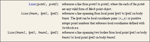
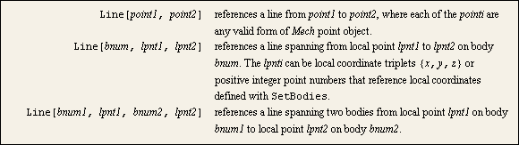
Any Mech function that calls for a vector object accepts either of the following syntax. 2DMethods of defining 2D vector objects. 3DMethods of defining 3D vector objects. Assuming that the appropriate body object definition has been made, any vector on any body can be referenced through either its global coordinates, its local coordinates, or its local point number. The following example shows several vector objects that are functionally identical. This defines some coordinates on the crank. Here are two identical vector specifications. 2.2.3 LinesThe Line object is used by Mech to reference a line in 2D or 3D space. A Line is defined two points: an origin point and an end point. The two points may be on the same or two different bodies. Because a Line object possesses both direction and location, it can be used in place of a vector object or an axis object in any Mech function that calls for a vector or an axis object.
Line objects have the same head as the built-in Mathematica Line graphics primitive. This does not lead to any conflict or require a redefinition of Line because it has no definition by default. The Line head is only used to hold its arguments in Mech, just as it is in standard Mathematica.
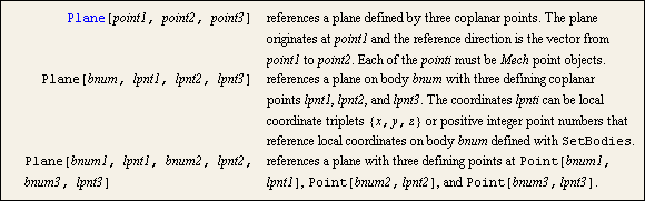
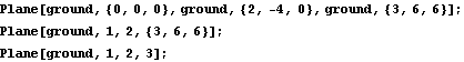
Any Mech function that calls for a vector or axis object accepts any of the following syntax. 2DMethods of defining 2D line objects. 3DMethods of defining 3D line objects. Assuming that the appropriate body object definition has been made, any line spanning bodies or on a single body can be referenced with a combination of global points, local points, or local point numbers. The following example shows several line objects that are functionally identical. This defines several points on the two bodies. Here are three identical line definitions. Here are two more identical line definitions. 2.2.4 PlanesThe Plane object is used by Modeler3D to reference a planar surface in 3D space. A Plane is defined by three points and has a specific origin, normal direction, and reference direction (see Axis). The first of the three points is the origin, and the vector from the first point to the second point is the reference direction. The third coplanar point cannot be colinear with the first two points. The positive normal is given by the cross product of the vector from the first point to the second point and the vector from the first point to the third point.
Because a Plane object possesses the properties of direction and location, it can be used in place of a vector object or an axis object in any Mech function that calls for a vector or an axis. If a Plane object is used to specify direction, the normal direction is used as the direction vector.
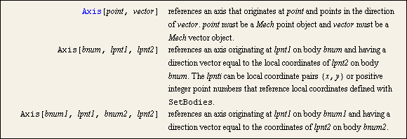
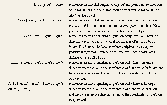
Any Modeler3D function that calls for a vector or axis object accepts any of the following syntax. 3DMethods of defining plane objects. Assuming that the appropriate body object definition has been made, a plane spanning any one, two, or three bodies can be referenced with a combination of global points, local points, or local point numbers. The following example shows several plane objects that are functionally identical. This loads the Modeler3D package. Local points are defined on the two bodies. Here are two identical plane definitions. Here are three more identical plane definitions. 2.2.5 Axes The axis object is used by Mech to reference an axis in 2D or 3D space. An axis object is specified by origin and direction. Optionally, 3D axis objects may have a reference direction specified. The reference direction is a vector that is not parallel to the direction of the axis. The reference direction is used by some Modeler3D constraints to control rotation about the axis.
An axis object may have the head Axis, Line, or Plane. If a Line is used to specify an axis object, the origin and direction of the Line are used as the origin and direction of the axis. Because a Line object has no specific reference direction, a Line should not be used in place of a Modeler3D axis object in a function where the reference direction is relevant.
If a Plane is used to specify an axis object, the origin of the Plane is used as the origin of the axis, the normal direction of the Plane is used as the direction of the axis, and the line from point1 to point2 on the Plane is used as the reference direction of the axis.
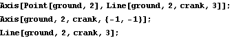
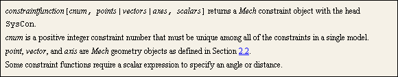
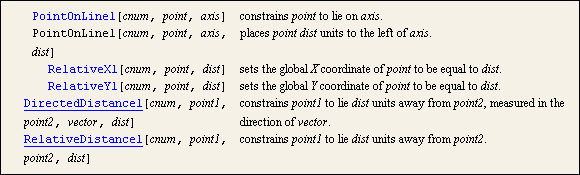
Any Mech function that calls for an axis object accepts any of the following syntax. 2DMethods of defining 2D axis objects. 3DMethods of defining 3D axis objects. Assuming that the appropriate body object definitions have been made, any axis with origin and direction specified with coordinates on a single body or multiple bodies can be referenced with a combination of global points, local points, or local point numbers. The following example shows several axis objects that are functionally identical. This loads the Modeler2D package. Local points are defined on the two bodies. Here are three functionally identical axis definitions. Here are three more identical axis definitions. 2.2.6 The Zeroth PointFor convenience, local point 0 (zero) can be used to reference the local origin of any body, although point 0 is never defined. The zeroth point can always be used, regardless of whether or not any SysBody objects have been defined and passed to SetBodies. The following examples show the use of the zeroth point. 2DHere are two identical 2D point objects. 3DHere are two identical 3D line objects. 2.3 Constraint ObjectsConstraint objects are used to define the mathematical relationships that make up the kinematic model in terms of the physical relationships of the various mechanism bodies. All Mech constraint functions return constraint objects with the head SysCon. These constraint objects are passed to the SetConstraints function to build the mathematical model. 2.3.1 General FormatAll arguments to any constraint function follow the same general format. Format for all constraint functions. Further, all constraint function names end with a single digit, except the general constraint function Constraint. This digit signifies the number of degrees of freedom constrained by the constraint. For example, the 2 in the Translate2 constraint function name signifies that it contains two constraint equations and constrains two degrees of freedom in a model. 2.3.2 2D Basic ConstraintsThe Modeler2D basic constraints specify elementary geometric relationships between points and lines on mechanism bodies. Elementary relationships are used for the majority of simple mechanical joints. A shaft spinning in a bearing is modeled by specifying that two points are coincident. A connecting rod can be modeled by specifying a constant distance between two points. A guide pin in a slot is modeled by specifying that a point on one body lies on a line on another body. A piston in a cylinder is modeled by specifying that two lines on two different bodies are colinear.
Many seemingly different mechanical joints are often modeled with the same constraint, such as a connecting rod versus a guide pin in a circular track; both are modeled by specifying the distance between two points on two different bodies. It is up to the user to determine the true nature of the kinematic relationships that make up a mechanism.
The entire set of Modeler2D constraint functions is quite redundant; all basic 2D mechanisms could, in fact, be modeled with a small subset of the Modeler2D constraints. The goal in this is to provide a constraint that is similar in form to the actual mechanical joint being modeled. Thus, the readability of the model can be improved.
Local coordinate constraints directly control the local coordinates of specified bodies. Point-on-line constraints force a point on a body to travel along a specified line. Point-at-position constraints force a point on a body to lie at a specified position. Angular constraints control the angle between the direction vectors of two lines. Compound constraints enforce multiple geometric relationships simultaneously. There are several other compound constraints available for modeling gears and cams, these are discussed in Chapter 6.
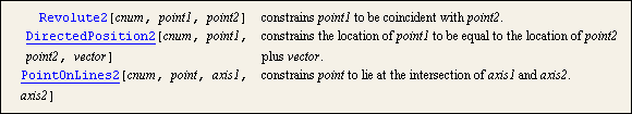
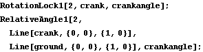
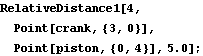
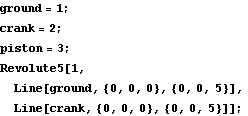
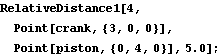
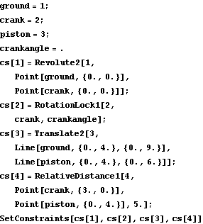
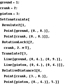
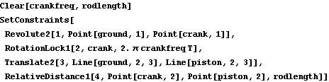
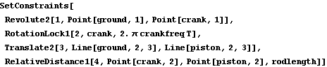
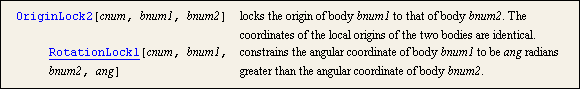
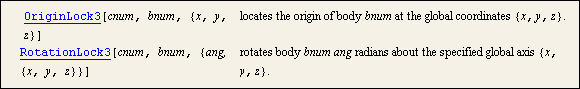
To demonstrate the ambiguity in determining which constraint is the correct constraint, the set of four constraints used in the crankshaft-piston model are examined. The first constraint, Revolute2, could be modeled with a pair of constraints with one degree of freedom each; a RelativeX1 to control the X coordinate of the crankshaft axis, and a RelativeY1 to control the Y coordinate. This loads the Modeler2D package. The Revolute2 constraint is functionally identical to a pair of one degree of freedom constraints. The second constraint, RotationLock1, could be modeled by constraining the angle between two lines, one on the crankshaft and one on the ground. Here are two equivalent constraints. The RelativeDistance1 constraint, in this application, cannot be replaced by the use of any other constraint. It is somewhat unique, geometrically. This constraint has no functional equivalent. 2.3.3 3D Basic ConstraintsThe Modeler3D basic constraints specify elementary geometric relationships between points, lines, and planes on mechanism bodies. Elementary relationships are used for the majority of mechanical joints. A shaft spinning in a bearing is modeled by specifying that two axes are coincident. A connecting rod can be modeled by specifying a constant distance between two points. A guide pin in a slot is modeled by specifying that a point on one body lies on a line on another body. A piston in a cylinder is modeled by specifying that two lines on two different bodies are colinear.
Many seemingly different mechanical joints are often modeled with the same constraint, such as a connecting rod versus a guide pin in a circular track; both are modeled by specifying the distance between two points on two different bodies. It is up to the user to determine the true nature of the kinematic relationships that make up a mechanism.
The entire set of Modeler3D constraint functions is quite redundant; all basic 3D mechanisms could, in fact, be modeled with a small subset of Modeler3D constraints. The goal in this is to provide a constraint that is similar in form to the actual mechanical joint being modeled. Thus, the readability of the model is improved.
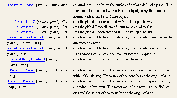
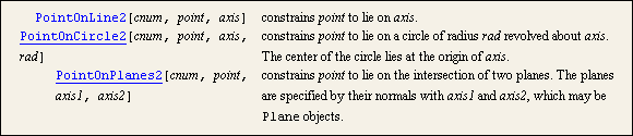
Local coordinate constraints directly control the local coordinates of specified bodies. Point-on-surface constraints force a point to lie on a specified surface. Point-on-line constraints force a point to lie on a line or curve. Point-at-position constraints control the position of a point. Angular constraints control the angle between two vectors. Parallel constraint enforces parallelism between two vectors. Constraints that enforce more complex geometric relationships. Compound constraints enforce multiple geometric relationships simultaneously. There are several other compound constraints available for modeling gears and cams; these are discussed in Chapter 6.
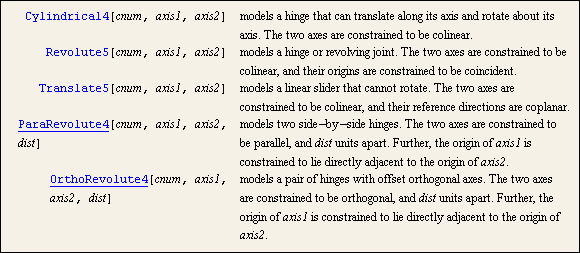
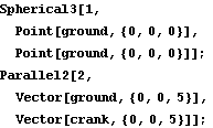
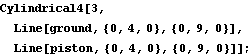
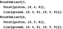
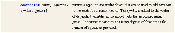
To demonstrate the ambiguity in determining which constraint is the correct constraint, the set of five constraints used in the crankshaft-piston model are reexamined. The first constraint, a Revolute5, could be modeled instead with two constraints; a Spherical3 constraint to control the position of the crankshaft, and a Parallel2 constraint to control the direction vector of the crankshaft's axis. This loads the Modeler3D package. Here is the original Revolute5 constraint. Here are an alternative pair of constraints that are functionally equivalent to the Revolute5 constraint. The third constraint, Cylindrical4, could be modeled by using two PointOnLine2 constraints. Here is the original Cylindrical4 constraint. Here are two constraints that are equivalent to the Cylindrical4 constraint. The RelativeDistance1 constraint in this application cannot be replaced by the use of any other constraint. It is somewhat unique, geometrically. This constraint has no functional equivalent. 2.3.4 The General ConstraintThe general constraint allows the user to enter a mathematical relationship directly as an equation. The general constraint function. For example, to constrain the origin of body 2 to lie on a paraboloid surface in the global coordinate system with its axis in the Z direction and Z intercept at {0, 0, 4}, Constraint would be used as follows. Here is a general mathematical constraint.
Out[22]= |  |
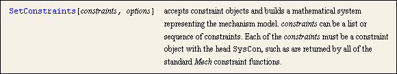
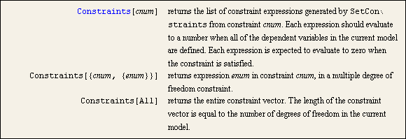
2.4 Building the ModelConstraint objects are processed into a kinematic model with the SetConstraints function. The system of equations generated by SetConstraints is not returned to the user; it is stored in several variables in Mech's private context. Thus only one mechanism model can be current in Mech at any given time. Several means of accessing and modifying the model are provided by Mech; these are discussed in the following section. 2.4.1 SetConstraintsSetConstraints is Mech's core model building function. SetConstraints takes constraint objects that represent the physical interactions in the mechanism model and processes them into a system of kinematic equations. The core model-building function. SetConstraints accepts options that determine how certain parts of the mathematical model are built. An option for SetConstraints. 2.4.2 ConstraintsThe actual constraint expressions that are generated by SetConstraints can be extracted with Constraints. Constraints can be very useful for debugging a model because it is often possible to read the constraint expressions directly and relate them to the function of the model. Constraints function. This loads the Modeler2D package. Consider the 2D crankshaft-piston model of Section 1.2. This model is built with various settings for the options for SetConstraints to show their affect on the resulting equations. Here is the crankshaft-piston model rebuilt. The first constraint cs[1] is a two degree of freedom constraint that constrains the origin of the crankshaft to lie at the global origin. Here is the expression generated by the Revolute2 constraint.
Out[11]= |  |
Obviously, when these two expressions are driven to zero, the desired result is achieved, the coordinates of the local origin of the crankshaft {X2, Y2} are zero.
The third constraint cs[3] is a two degree of freedom constraint that allows the piston to translate along a vertical axis, but constrains its rotation and its translation in the X direction. Here is the expression generated by the Translate2 constraint.
Out[12]= |  |
The first expression, 10 Sin[3], constrains the rotation of the piston; this expression can be equal to zero if 3 is any integer multiple of  . The reason that the solution 3 -> 0 is found is because the default initial guess is 3 -> 0. If a different initial guess were used, such as 3 -> 3, the model would converge to 3 -> N[] instead. . The reason that the solution 3 -> 0 is found is because the default initial guess is 3 -> 0. If a different initial guess were used, such as 3 -> 3, the model would converge to 3 -> N[] instead.
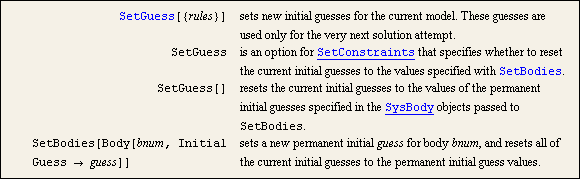
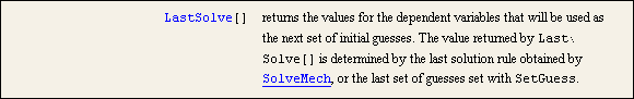
The second expression in the list constrains the X coordinate of the piston to be zero. Notice that at any value of 3 that satisfies the first expression, the second expression reduces to  or or  , either of which will drive X3 to zero. , either of which will drive X3 to zero. 2.4.3 Initial GuessesSetGuess serves both as an option for several Mech functions, and as a function for temporarily setting a model's initial guesses. Various methods of setting initial guesses. A SolveMech utility. To advance the position for the model in large steps, it is sometimes necessary to specify a better initial guess than the current one. For example, to turn the crankshaft 3/4 of a turn at once, it might be necessary to set a new initial guess for 2 and Y3, the angular coordinate of the crankshaft and the height of the piston, respectively. This runs the model at its initial position.
Out[14]= |  |
This sets new guesses for 2 and Y3.
Out[15]= |  |
This runs the model at 3/4 turn of the crank.
Out[17]= |  |
If SetConstraints were to be run at this time with the default options, the initial guesses would remain at their current values,  and and  . The SetGuess option resets the guesses to their defaults. . The SetGuess option resets the guesses to their defaults. The SetGuess option resets the initial guesses. This shows the current guesses.
Out[20]= |  |
2.4.4 $MechProcessFunction$MechProcessFunction is a function that is applied to all of the mechanism equations that are generated by SetConstraints as they are created. The default setting, $MechProcessFunction = Chop, can reduce the size of the constraint expressions substantially if any of the constraints involve the local origins of bodies in the model which have local coordinates of  or or  . Setting $MechProcessFunction = Identity disables this action. . Setting $MechProcessFunction = Identity disables this action. Set $MechProcessFunction equal to Identity to disable chopping. Here the model is built without chopping the constraints. Here is the Revolute2 constraint.
Out[23]= |  |
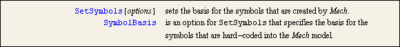
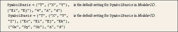
Obviously, the run time of the model is increased by increasing the size of the constraint expressions. However, if the model contains very small physical dimensions, it may not be acceptable to apply Chop to the constraints. 2.4.5 SetSymbolsThe default symbols that appear in the solution rules returned by SolveMech can be changed with the SetSymbols function. A model set-up function. Default settings. Because SetSymbols changes the behavior of all Mech functions that return symbolic expressions, SetSymbols must be run before building any other part of the mechanism model with SetBodies or SetConstraints. SetSymbols has the effect of executing ClearMech[].
The  x, y, and z symbols are used by Modeler3D to represent angular velocities used in 3D velocity analysis, which is discussed in Chapter 4. The x, y, and z symbols are used by Modeler3D to represent angular velocities used in 3D velocity analysis, which is discussed in Chapter 4. The  symbol is a Lagrange multiplier used in static and dynamic analysis, which is discussed in Chapter 7. The d symbol is used in 2D and 3D velocity analysis to symbolically represent differentiation. symbol is a Lagrange multiplier used in static and dynamic analysis, which is discussed in Chapter 7. The d symbol is used in 2D and 3D velocity analysis to symbolically represent differentiation.
If the current model is rebuilt with a new setting for SymbolBasis, the solution rules returned by SolveMech are changed accordingly. This causes new symbols to be used in all subsequent models. The model is rebuilt with SetConstraints. This runs the model at crankangle = 0.5.
Out[28]= |  |
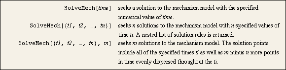
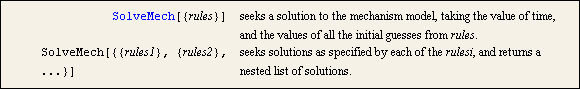
This returns MechanicalSystems to its initial state. 2.5 Running the ModelThis section covers the use of the SolveMech command, which is used to seek a solution to the mechanism model. The Mech commands covered in the previous sections were all concerned with building a mechanism model. SolveMech is the sole function for running the model. 2.5.1 SolveMechThe SolveMech command is used without arguments to seek a single solution to the mechanism model, with all of the current values of any user-defined variables in the model. When SolveMech seeks a solution, what it is really trying to do is numerically find the location and orientation of each of the bodies in the model at which all of the constraints are satisfied. Mech's runtime command. Time DependenceMost mechanism models have some dependency on time that is specified (by default) by the symbol T. When T appears in a mechanism model, the model's location becomes explicitly a function of time, a technique that must be used in the velocity and acceleration portions of the analysis. It is not necessary to have any dependency on T in a model used only for location analysis, but it is customary to make the primary driving expression a function of T anyway. The symbol for time. SolveMech has several special invocations that are useful for finding a solution or many solutions at a range of values of T. More arguments for SolveMech. The 2D crankshaft-piston model is used to demonstrate the various forms of SolveMech. When this example was first used in Section 1.2, the symbol crankangle was used to specify the rotation of the crankshaft. Now crankangle is replaced with  so that the rotation of the crankshaft is a function of time. Thus, the crankshaft has an angular velocity of one revolution per second. so that the rotation of the crankshaft is a function of time. Thus, the crankshaft has an angular velocity of one revolution per second. This loads the Modeler2D package. Here is the crankshaft-piston model with a time-dependent driver. Now, instead of changing the value of crankangle to drive the model the value of time is changed directly with SolveMech. This runs the model at 1/10 turn of the crankshaft.
Out[6]= |  |
This seeks 3 solutions from 0 to 0.5 turns, inclusive.
Out[7]= |  |
The unusual form of the iteration specifier in SolveMech is very useful if an even spread of data is desired, with a few particular data points specified in between. For example, the following example generates six solution points with the points T = 0., 0.223, and 0.3 included, and the other three points spread so as to fill the gaps as evenly as possible. This seeks 6 solution points, including T = 0.223
Out[8]= |  |
Initial Guesses at RuntimeSetting initial guesses with SolveMech. The primary reason for passing rules into SolveMech, instead of just specifying the value of time, is to accelerate the solution process. The supplied rules may be known to be very good initial guesses, such as rules obtained from a prior run with a slightly different value for a parameter. This calls SolveMech with a list of guesses. The value of time T = 0.2 is pulled from the guesses.
Out[9]= |  |
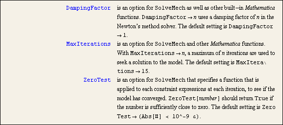
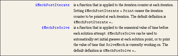
2.5.2 Controlling SolveMechThe nonlinear equation solver used by SolveMech can be controlled by setting the values of several options. Many of these options are the same as those used by FindRoot, although SolveMech does not utilize FindRoot. Options for SolveMech. The operation of SolveMech can be inspected by the use of two hook functions that are called during the execution of SolveMech. Note that all Mech system variables that can be set by the user have names of the form "$Mech*". Controls for SolveMech. Failure to ConvergeThe default setting for ZeroTest will suffice for many models, but may need to be changed for several reasons.
If the numerical size of the dimensions of the model are very large or small, ZeroTest may need to be changed accordingly. For example, if a typical point in the model is Point[2, {3400, -7800}], it might be necessary to specify ZeroTest -> (Abs[#] < 10^-6 &).
If the model is large (eight or more bodies for 2D, four or more for 3D) solving the linear equations at each iteration begins to suffer from numerical error. Thus, it may be necessary to lower the convergence criteria.
The primary indication that the convergence criteria must be changed is that SolveMech returns a valid solution that is apparently correct, but an error message is generated claiming that convergence has failed after n iterations. If the model fails to converge and returns a solution that is obviously not valid, try to find an inconsistency in the constraint set or consult Chapter 13, Debugging Models. 2.5.3 Nonlinear Equation SolverAt the core of Mech's numerical solution block is a Newton-Rhapson simultaneous nonlinear equation solver, similar to the built-in Mathematica function FindRoot. In fact, Mech can be used to solve arbitrary systems of equations that have no relation to mechanism analysis.
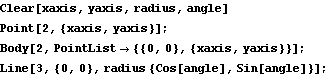
Mech's general constraint function Constraint is used to build a constraint object from an arbitrary algebraic equation. The algebraic constraint can be incorporated into a mechanism model along with other geometric constraints, or an entire model can be built from general constraints. The general constraint function. The following uses Mech to find the intersection of a parabola and a circle. This prevents impending spelling errors. This builds the nonmechanical model. This plots the two functions, showing their intersection.
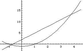
Out[14]= |  |
This seeks a solution to the two equations.
Out[15]= | 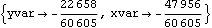 |
This looks for the other solution.
Out[16]= | 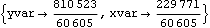 |
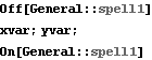
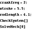
2.6 Variable ManagementMechanism models often need to have many adjustable parameters that can be tweaked between runs of the model. A Mech model may have any number of user-defined variables, provided that all such variables in a model have numerical values before SolveMech is called. 2.6.1 User-Defined VariablesThis loads the Modeler2D package. Symbolic parameters can enter a kinematic model in two ways. The coordinates of a local point can be given in symbolic form or the arguments of a constraint function that specify a distance or angle can be given as a symbolic expression. The following example shows how local point specifications can be symbolic. This prevents impending spell check warnings. All local coordinates can be specified symbolically. The crankshaft-piston model can be built with several variables in the arguments to its constraint functions. The following example introduces symbols into the model to represent the frequency of the crankshaft rotation, the length of the connecting rod, and the stroke of the crankshaft. Here are the crankshaft-piston body objects, with a symbol included in the points list. This builds the constraint equations with two symbols embedded. If SolveMech is called now to seek a solution, an error message is generated because some of the symbols in the model have not yet been defined. This attempts to find a solution.

Out[19]= |  |
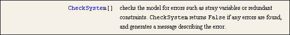
A debugging aid. CheckSystem reports the names of any undefined symbols, as well as several other possible errors in the model. This checks the integrity of the model.
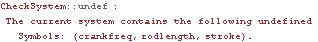
Out[20]= |  |
This defines the undefined symbols, checks the model, and runs it.
Out[24]= |  |
Out[25]= |  |
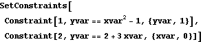
Dependent Variables It is acceptable to use Mech dependent variables explicitly when defining local points or constraints. Highly abstract compound constraints can be specified in this manner. This is an extremely obtuse constraint. This constraint would cause the Y coordinate of a point on body 2 to be equal to the X coordinate of the origin of body 3, squared. When using dependent variables in constraints, care must be taken to ensure that the dependence of the constraint on the variables is explicit at the time that SetConstraints is run. If not, differentiation with respect to those variables cannot occur, and the constraints will not be processed correctly.
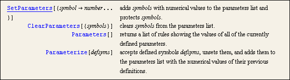
Note that the names of the dependent variables used by Mech are cleared and protected when SetConstraints is run. Thus, if there happens to be a definition in place such as Y2 = 3, it is removed by SetConstraints. 2.6.2 ParametersAnother method of managing variables in a Mech model is to use the parameters functions. The parameters list is basically a list of rules stored in Mech's internal database that is applied to the mechanism model immediately before the solution phase. By using parameters, problems can be avoided such as failing to define all of the symbols in a model or accidentally defining them before SetConstraints is run and hard coding them into the model. Parameter management functions. Note that when a parameter is set with SetParameters or Parameterize, it is protected until it is unset with ClearParameters. This is to ensure that the parameter cannot be accidentally given a definition in the course of running the model.
The crankshaft-piston model, which was built in Section 2.6.1, is used to demonstrate the use of parameters. The definitions of the three symbols in the model are cleared and then added to the parameters list. This adds three symbols to the parameters list.
Out[28]= |  |
The crankshaft-piston model can now be built without worrying about the definitions of the parameters. SetParameters can be used at any time in the model-building process. Here the crankshaft-piston model is rebuilt with reference to the body objects previously defined. The parameters are included in the solution rules returned by SolveMech.
Out[30]= |  |
Set a new value for crankfreq. Only the specified value is updated, the others are left unchanged.
Out[31]= |  |
The parameters are protected.

This removes all of the parameters from the parameters list.
Out[33]= |  |
|