Heat Conduction in a Multilayer Sphere

Introduction	Solve the PDE Heat Transfer Model
Domain and Mesh Generation	Post-processing and Visualization
Heat Transfer Model	Nomenclature
Initial and Boundary Conditions	References

Introduction

Devices constructed by layers of multiple materials have been used in many industrial applications, such as chemical, mechanical and aerospace engineering. One important feature of multilayered materials lies in the possibility to combine several thermal properties. Performing numerical simulations and obtaining the temperature distribution of such compounds are important because they give insights into how the real system will behave.

This model is based on [Singh et al., 2016] in which a 3D heat transfer transport through a multilayered sphere was analyzed. The problem statement is to perform a thermal analysis and find the temperature field distribution at time of concentric hollow spherical layers in thermal contact. A 2D cross section of the geometry is shown for .

Each layer of the sphere has specific material properties; for example, the ^th layer will have a thermal conductivity , mass density and specific heat capacity . This simulation is limited to three layers—three concentric hollow spheres—and . As mentioned in [Singh et al., 2016], two different types of boundary conditions are imposed, one at the external face and a second type at the internal face of the multilayer sphere setup. In this model, the external face of the hollow sphere is subjected to a nonlinear heat source at all times, and the internal face of the first layer will be set to a fixed temperature of . The simulation starts with an initial temperature of for all layers of the sphere. As heat transfers between layers, the temperature change of each layer will depend, as expected, on its thermal properties.

Refer to the information provided in Heat Transfer for a more general theoretical background on heat transfer analysis.

Load the Finite Element package and OpenCascadeLink:

Domain and Mesh Generation

The following plot shows a two-dimensional cross sectional cut through the three concentric spherical layers. Indicated are the radii r_i and the model parameter labels of each layer , and .

Specify the values of the radii for each layer:

Use functions from OpenCascadeLink to generate four concentric balls:

Convert the shapes to faces to define internal boundaries in the geometry:

Next, the faces are combined. This will result in an object with four regions, , . The multilayered sphere is hollow in the region . This requirement can be specified during the mesh generation with the ToElementMesh option RegionHoles.

Define an object with four faces and four regions:

Generate the boundary mesh:

The three layers will be labeled with three markers 1, 2 and 3. For more information on markers and their generation in meshes, see the "Element Mesh Generation" tutorial.

Relate layer names to the markers:

Create a full ElementMesh:

Heat Transfer Model

A transient heat transfer equation (1) will be used to determine the temperature field distribution :

For this PDE model, two boundary conditions will be applied to the inner face () and the external face () of the multilayer sphere. On the inner face, a surface boundary condition of constant temperature equal to will be imposed. On the external face, a nonlinear heat flux source of value will be imposed, where is the polar angle and is the azimuthal angle in spherical coordinates.

Define the material parameters of the model by layer:

Define a helper function to specify the material parameters for each layer with the use of ElementMarker:

Also, see this note about how to set up of computationally efficient PDE coefficients.

Define the heat transfer model parameters for all the geometry:

Set up the model variables vars and parameters pars of the model:

Initial and Boundary Conditions

For this PDE model, the internal face of layer 1 will be set to a temperature surface boundary condition of c. The external face of layer 3 will be subjected to a nonuniform time-independent heat flux condition that depends on the polar angle and the azimuthal angle . The problem description in [Singh et al., 2016] is formulated in spherical coordinates. To apply the boundary conditions, originally defined in spherical coordinates, a coordinate transformation from spherical coordinates to Cartesian coordinates is performed.

Define transformation rules from spherical to Cartesian coordinates:

Specify

, the heat source magnitude, and convert the original boundary conditions to Cartesian coordinates:

First, a DirichletCondition is set up with the help of the HeatTemperatureCondition function.

Set the temperature

at all times at

The NeumannValue on the outside of the sphere is created with the help of the HeatFluxValue function. The heat-flux source is applied on the external face of layer 3.

Create the heat flux on the outside where

, and for

and

Set up the initial temperature of the multilayer sphere to

The following plot shows the heat flux boundary condition and the coordinate system used to formulate the problem. The heat flux has its peak value at , and it decreases to 0 in the region :

Solve the PDE Heat Transfer Model

To analyze the heat conduction between the three layers, the model is solved from to .

Define the initial and final time of integration:

Define the heat transfer equation to solve with the use of the HeatTransferPDEComponent:

Solve the heat transfer PDE model and monitor the time/memory usage:

Post-processing and Visualization

Next, 1D, 2D and 3D cuts of the temperature field distribution of the multilayered sphere are visualized.

1-Dimensional Cut: Temperature Distribution in Radial Direction

The transient temperature distribution solutions are plotted in the radial direction along and the azimuthal () directions: a) , b) and c) .

Define the times for which the temperature will be plotted:

The linear section corresponds to , corresponds to , and corresponds to .

Define the radial cuts of the multilayer sphere for the plots in the directions of

Generate the time legend values:

Plot the temperature field in the three radial cuts:

Show the solutions:

2-Dimensional Cut: Temperature Contour Plot Distribution

Visualize the temperature field contours in the cross section of the sphere. The temperature distribution of the whole system increases with time. For each time in , a list of nine temperature values is defined to plot as contours.

Create six lists of nine temperature contour values for each time t and relate them with the times list:

Construct the cross section of the multilayer sphere:

Color style of contour lines:

Define a function that uses ContourPlot and plots the temperature field at time

Display the plots in an array:

Show all contour plots at different times:

3-Dimensional Cut: Temperature Density Plot Animation

A time animation is performed of the temperature field distribution in a 3D section of the sphere. When the heat source is applied from the region , the temperature starts to increase in the direction, as can be seen in the animation below. Since the relationship between thermal conductivities of each layer is , layer 3 (outer layer) transports heat and increases its temperature faster than the internal layer, as can be seen in the density plot animation.

Define the temperature range values and the legend bar format with BarLegend:

A limit in the plot range of the SliceContourPlot3D is used, and the reason is that if the center sphere of the slice surface "CenterCutSphere" is exactly the same sphere as the region of the mesh it is plotted over, part of the surface will not be displayed. Therefore, the range of the plot must be smaller than the region of the mesh.

Define the plot range limit and the density plot options:

The 3D animations that follow can require an above-average amount of disk space. To reduce the disk space this notebook requires, the function Rasterize is called on the visualization. The disadvantage of this is that the quality of the animation will not be as sharp as without it. To obtain high-quality graphics, remove the call to Rasterize.

Show the animation:

Nomenclature

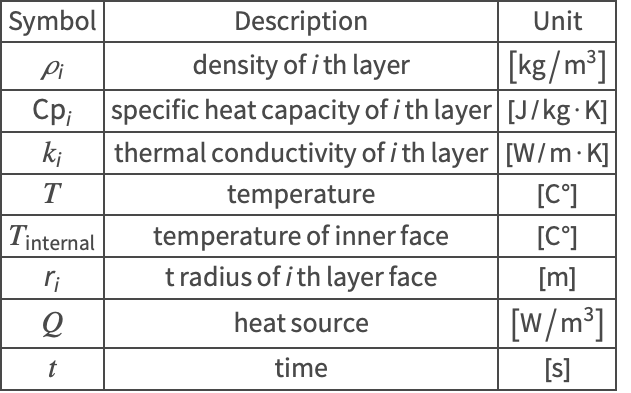
References

1. Suneet, S., Jain, P. K. and Uddin, R. "Analytical Solution for Three-Dimensional, Unsteady Heat Conduction in a Multilayer Sphere." ASME Journal of Heat Transfer, 2016, 138(10), 101301. doi: 10.1115/1.4033536.

Top