AcousticPDEComponent[vars,pars]
生成变量为 vars 且参数为 pars 的偏微分方程声学项分量.
AcousticPDEComponent
AcousticPDEComponent[vars,pars]
生成变量为 vars 且参数为 pars 的偏微分方程声学项分量.
更多信息
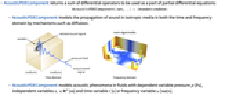
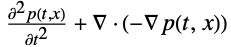
- AcousticPDEComponent 返回微分算子的总和,以用作偏微分方程的一部分:
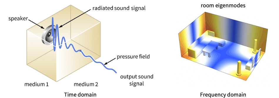
- AcousticPDEComponent 在时域和频域中对声音通过扩散等机制在各向同性介质中的传播进行建模.
- AcousticPDEComponent 使用以 [
] 为单位的因变量压力
、以 [
] 为单位的自变量
、以 [
] 为单位的时间变量
和以 [
] 为单位的频率变量
为液体中声学现象建模. - 与时间相关的变量 vars 为 vars={p[t,x1,…,xn],t,{x1,…,xn}}.
- 与频率相关的变量 vars 为 vars={p[x1,…,xn],ω,{x1,…,xn}}.
- 时域声学模型 AcousticPDEComponent 基于如下波动方程,其中时间变量为
,密度为
,声速为
,声源为
和
: - 频域声学模型 AcousticPDEComponent 基于角频率为
的亥姆霍兹方程: - 偏微分方程声学项的单位为 [1/
]. - 可以给出以下参数 pars:
-
参数 缺省值 符号 "DipoleSource" {0,…}
,偶极子声源,单位为 [
]"MassDensity" 1
,介质密度,单位为 [
]"Material" Automatic 
"MonopoleSource" 0
,单极子声源,单位为 [1/
]"RegionSymmetry" None 
"SoundSpeed" 1
,声速,单位为 [
] - 所有参数可能取决于
、
和
以及其他因变量中的任何一个,除了
以外,从而导致非线性特征值问题. - AcousticPDEComponent 允许时域中的声源和频域中的声源.
-
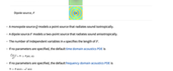
单极子声源, 
Wolfram Language code: [image]偶极子声源, 
Wolfram Language code: [image] - 单极子声源
模拟点声源,它以各向同性方式辐射声音. - 偶极子声源
模拟两点源,它以各向异性方式辐射声音.
中自变量的数量指定
的长度.- 如果未指定任何参数,则默认时域声学偏微分方程为
- 如果未指定任何参数,则默认频域声学偏微分方程为
- 参数 "RegionSymmetry" 的一个可能选择是 "Axisymmetric".
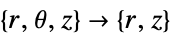
- "Axisymmetric" 区域对称性代表了一个截断的圆柱坐标系,其中圆柱坐标通过去除角度变量而约化,如下所示:
-
维度 约化 方程式 一维 
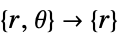

二维 

- 如果 AcousticPDEComponent 取决于在关联 pars 中指定为 …,keypi…,pivi,… 的参数
,则参数
用
代替.
范例
打开所有单元 关闭所有单元基本范例 (4)
AcousticPDEComponent[{p[t, x], t, {x}}, <||>]AcousticPDEComponent[{p[x], ω, {x}}, <||>]vars = {p[t, x], t, {x}};
pars = <|"SoundSpeed" -> 343, "MassDensity" -> 1.2|>;p0 = D[0.125 Erf[(x - 0.5) / 0.15], x];
ics = {p[0, x] == p0, Derivative[1, 0][p][0, x] == -343 * D[p0, x]};eqn = AcousticPDEComponent[vars, pars] == AcousticSoundHardValue[x == 1, vars, pars]pfun = NDSolveValue[{eqn, ics}, p, {t, 0, 0.003}, x∈Line[{{0}, {1}}]];Manipulate[Plot[pfun[t, x], {x, 0, 1}, ...], {{t, 0}, 0, 0.003, 10 ^ -4}, Rule[...]]vars = {p[x], ω, {x}};
pars = <|"SoundSpeed" -> 343, "MassDensity" -> 1.2|>;eqn = AcousticPDEComponent[vars, pars] == AcousticRadiationValue[x == 0, vars, pars, <|"SoundIncidentPressure" -> 1|>];pfun = ParametricNDSolveValue[eqn, p, x∈Line[{{0}, {1}}], {ω}];Plot[Table[Legended[Abs[pfun[ω][x]], ω], {ω, {1000π, 1500π, 2000π}}]//Evaluate, {x, 0, 1}, ...]范围 (21)
基本用法 (2)
时域 (7)
vars = {p[t, x], t, {x}};
pars = <|"SoundSpeed" -> 343, "MassDensity" -> 1.2|>;p0 = D[0.125 Erf[(x - 0.5) / 0.15], x];
ics = {p[0, x] == p0, Derivative[1, 0][p][0, x] == -343 * D[p0, x]};eqn = AcousticPDEComponent[vars, pars] == AcousticAbsorbingValue[x == 1, vars, pars];pfun = NDSolveValue[{eqn, ics}, p, {t, 0, 0.003}, x∈Line[{{0}, {1}}]];Manipulate[Plot[pfun[t, x], {x, 0, 1}, ...], {{t, 0.0013}, 0, 0.003, 10 ^ -4}, Rule[...]]vars = {p[t, x], t, {x}};
pars = <|"SoundSpeed" -> 317, "MassDensity" -> 1.41|>;p0 = D[0.125 Erf[(x - 0.5) / 0.15], x];
ics = {p[0, x] == p0, Derivative[1, 0][p][0, x] == -317 * D[p0, x]};eqn = AcousticPDEComponent[vars, pars] == AcousticImpedanceValue[x == 1, vars, <|"SpecificAcousticImpedance" -> 287.33|>];pfun = NDSolveValue[{eqn, ics}, p, {t, 0, 0.003}, x∈Line[{{0}, {1}}]];Manipulate[Plot[pfun[t, x], {x, 0, 1}, ...], {{t, 0.0006}, 0, 0.003, 10 ^ -4}, Rule[...]]vars = {p[t, x], t, {x}};
pars = <|"SoundSpeed" -> 343, "MassDensity" -> 1.2|>;ics = {p[0, x] == 0, Derivative[1, 0][p][0, x] == 0};eqn = AcousticPDEComponent[vars, pars] == AcousticNormalVelocityValue[x == 0, vars, pars, <|"AcousticSoundParticleVelocity" -> Sin[800π t]|>];pfun = NDSolveValue[{eqn, ics}, p, {t, 0, 0.0025}, x∈Line[{{0}, {1}}], Method -> {"PDEDiscretization" -> {"MethodOfLines", "SpatialDiscretization" -> {"FiniteElement", "MeshOptions" -> {"MaxCellMeasure" -> 0.015}}}}];Manipulate[Plot[pfun[t, x], {x, 0, 1}, ...], {{t, 0.0012}, 0, 0.0025, 10 ^ -4}, Rule[...]]vars = {p[t, x], t, {x}};
pars = <|"SoundSpeed" -> 343, "MassDensity" -> 1.2|>;ics = {p[0, x] == 0, Derivative[1, 0][p][0, x] == 0};eqn = {AcousticPDEComponent[vars, pars] == 0, AcousticPressureCondition[x == 0, vars, pars, <|"AcousticPressure" -> Sin[800π t]|>]};pfun = NDSolveValue[{eqn, ics}, p, {t, 0, 0.0025}, x∈Line[{{0}, {1}}], Method -> {"PDEDiscretization" -> {"MethodOfLines", "SpatialDiscretization" -> {"FiniteElement", "MeshOptions" -> {"MaxCellMeasure" -> 0.015}}}}];Manipulate[Plot[pfun[t, x], {x, 0, 1}, ...], {{t, 0.001}, 0, 0.0025, 10 ^ -4}, Rule[...]]vars = {p[t, x], t, {x}};
pars = <|"SoundSpeed" -> 343, "MassDensity" -> 1.2|>;ics = {p[0, x] == 0, Derivative[1, 0][p][0, x] == 0};eqn = AcousticPDEComponent[vars, pars] == AcousticRadiationValue[x == 0, vars, pars, <|"SoundIncidentPressure" -> Sin[800π t]|>];pfun = NDSolveValue[{eqn, ics}, p, {t, 0, 0.01}, x∈Line[{{0}, {1}}]];Manipulate[Plot[pfun[t, x], {x, 0, 1}, ...], {{t, 0.0074}, 0, 0.01, 10 ^ -4}, Rule[...]]vars = {p[t, x], t, {x}};
pars = <|"SoundSpeed" -> 343, "MassDensity" -> 1.2|>;p0 = D[0.125 Erf[(x - 0.5) / 0.15], x];
ics = {p[0, x] == p0, Derivative[1, 0][p][0, x] == -343 * D[p0, x]};eqn = AcousticPDEComponent[vars, pars] == AcousticSoundHardValue[x == 1, vars, pars];pfun = NDSolveValue[{eqn, ics}, p, {t, 0, 0.003}, x∈Line[{{0}, {1}}]];Manipulate[Plot[pfun[t, x], {x, 0, 1}, ...], {{t, 0.0016}, 0, 0.003, 10 ^ -4}, Rule[...]]vars = {p[t, x], t, {x}};
pars = <|"SoundSpeed" -> 343, "MassDensity" -> 1.2|>;p0 = D[0.125 Erf[(x - 0.5) / 0.15], x];
ics = {p[0, x] == p0, Derivative[1, 0][p][0, x] == -343 * D[p0, x]};eqn = {AcousticPDEComponent[vars, pars] == 0, AcousticSoundSoftCondition[x == 1, vars, pars]};pfun = NDSolveValue[{eqn, ics}, p, {t, 0, 0.003}, x∈Line[{{0}, {1}}]];Manipulate[Plot[pfun[t, x], {x, 0, 1}, ...], {{t, 0.0022}, 0, 0.003, 10 ^ -4}, Rule[...]]频域 (10)
AcousticPDEComponent[{p[x], ω, {x}}, <|"SoundSpeed" -> c, "MassDensity" -> ρ|>]AcousticPDEComponent[{p[x], ω, {x}}, <|"Material" -> Entity["Element", "Argon"]|>]AcousticPDEComponent[{p[x], ω, {x}}, Entity["Element", "Argon"]]vars = {p[x], ω, {x}};
pars = <|"SoundSpeed" -> 343, "MassDensity" -> 12 / 10|>;eqn = AcousticPDEComponent[vars, pars] == AcousticRadiationValue[x == 0, vars, pars, <|"SoundIncidentPressure" -> 1|>] + AcousticAbsorbingValue[x == 1, vars, pars]pfun = ParametricNDSolveValue[eqn, p, x∈Line[{{0}, {1}}], {ω}];Plot[Table[Legended[Abs[pfun[ω][x]], ω], {ω, {1000π, 1500π, 2000π}}]//Evaluate, {x, 0, 1}, ...]Plot[Table[Legended[Re[pfun[ω][x] * Exp[I ω t]], ω], {t, {0.01}}, {ω, {1000π, 1500π, 2000π}}]//Evaluate, {x, 0, 1}, ...]vars = {p[x], ω, {x}};
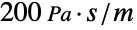
pars = <|"SoundSpeed" -> 343, "MassDensity" -> 1.2|>;eqn = AcousticPDEComponent[vars, pars] == AcousticRadiationValue[x == 0, vars, pars, <|"SoundIncidentPressure" -> 1|>] + AcousticImpedanceValue[x == 1, vars, pars, <|"SpecificAcousticImpedance" -> 200|>];pfun = ParametricNDSolveValue[eqn, p, x∈Line[{{0}, {1}}], {ω}];Plot[Table[Legended[Abs[pfun[ω][x]], ω], {ω, {1000π, 1500π, 2000π}}]//Evaluate, {x, 0, 1}, ...]Plot[Table[Legended[Re[pfun[ω][x] * Exp[I ω t]], ω], {t, {0.01}}, {ω, {1000π, 1500π, 2000π}}]//Evaluate, {x, 0, 1}, ...]vars = {p[x], ω, {x}};
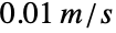
pars = <|"SoundSpeed" -> 343, "MassDensity" -> 1.2|>;建立方程,左端有一个声学法向速度边界,声粒子速度
为
,右端有一个吸声边界:
eqn = AcousticPDEComponent[vars, pars] == AcousticNormalVelocityValue[x == 0, vars, pars, <|"AcousticSoundParticleVelocity" -> 0.01|>] + AcousticAbsorbingValue[x == 1, vars, pars];pfun = ParametricNDSolveValue[eqn, p, x∈Line[{{0}, {1}}], {ω}];Manipulate[Plot[Abs[pfun[ω][x]], {x, 0, 1}, ...], {{ω, 1000π, "f"}, {1000π, 1500π, 2000π}}, Rule[...]]Manipulate[Plot[Re[pfun[ω][x] * Exp[I ω t]], {x, 0, 1}, ...], {{t, 0, "t"}, 0, 0.01}, {{ω, 1000π, "f"}, {1000π, 1500π, 2000π}}, Rule[...]]vars = {p[x], ω, {x}};
pars = <|"SoundSpeed" -> 343, "MassDensity" -> 1.2|>;eqn = AcousticPDEComponent[vars, pars] == AcousticPressureCondition[x == 0, vars, pars, <|"AcousticPressure" -> 1|>] + AcousticAbsorbingValue[x == 1, vars, pars];pfun = ParametricNDSolveValue[eqn, p, x∈Line[{{0}, {1}}], {ω}];Manipulate[Plot[Abs[pfun[ω][x]], {x, 0, 1}, ...], {{ω, 1000π, "f"}, {1000π, 1500π, 2000π}}, Rule[...]]Manipulate[Plot[Re[pfun[ω][x] * Exp[I ω t]], {x, 0, 1}, ...], {{t, 0, "t"}, 0, 0.01}, {{ω, 1000π, "f"}, {1000π, 1500π, 2000π}}, Rule[...]]vars = {p[x], ω, {x}};
pars = <|"SoundSpeed" -> 343, "MassDensity" -> 1.2|>;eqn = AcousticPDEComponent[vars, pars] == AcousticRadiationValue[x == 0, vars, pars, <|"SoundIncidentPressure" -> 1|>];pfun = ParametricNDSolveValue[eqn, p, x∈Line[{{0}, {1}}], {ω}];Plot[Table[Legended[Abs[pfun[ω][x]], ω], {ω, {1000π, 1500π, 2000π}}]//Evaluate, {x, 0, 1}, ...]Plot[Table[Legended[Re[pfun[ω][x] * Exp[I ω t]], ω], {t, {0.01}}, {ω, {1000π, 1500π, 2000π}}]//Evaluate, {x, 0, 1}, ...]vars = {p[x], ω, {x}};
pars = <|"SoundSpeed" -> 343, "MassDensity" -> 1.2|>;建立方程,其左端为声辐射边界,压力源
为
,右端为声学硬边界:
eqn = AcousticPDEComponent[vars, pars] == AcousticSoundHardValue[x == 1, vars, pars] + AcousticRadiationValue[x == 0, vars, pars, <|"SoundIncidentPressure" -> 1|>];pfun = ParametricNDSolveValue[eqn, p, x∈Line[{{0}, {1}}], {ω}];Plot[Table[Legended[Abs[pfun[ω][x]], ω], {ω, {1000π, 1500π, 2000π}}]//Evaluate, {x, 0, 1}, ...]Plot[Table[Legended[Re[pfun[ω][x] * Exp[I ω t]], ω], {t, {0.01}}, {ω, {1000π, 1500π, 2000π}}]//Evaluate, {x, 0, 1}, ...]vars = {p[x], ω, {x}};
pars = <|"SoundSpeed" -> 343, "MassDensity" -> 1.2|>;eqn = {AcousticPDEComponent[vars, pars] == AcousticRadiationValue[x == 0, vars, pars, <|"SoundIncidentPressure" -> 1|>], AcousticSoundSoftCondition[x == 1, vars, pars]};pfun = ParametricNDSolveValue[eqn, p, x∈Line[{{0}, {1}}], {ω}];Plot[Table[Legended[Abs[pfun[ω][x]], ω], {ω, {1000π, 1500π, 2000π}}]//Evaluate, {x, 0, 1}, ...]Plot[Table[Legended[Re[pfun[ω][x] * Exp[I ω t]], ω], {t, {0.01}}, {ω, {1000π, 1500π, 2000π}}]//Evaluate, {x, 0, 1}, ...]单位 (2)
应用 (1)
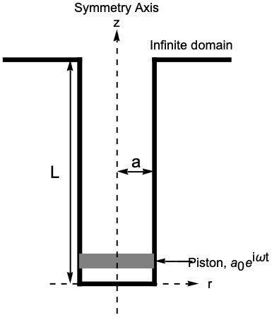
下面的声学模型描述了一个开放式管道,在管道的一端放置了一个振动活塞,而管道的另一端则通向一个无限域. 在这种情况下,在一端设置一个阻抗边界条件来模拟无限域. 要模拟的管道是一个法兰圆管,如下图所示:
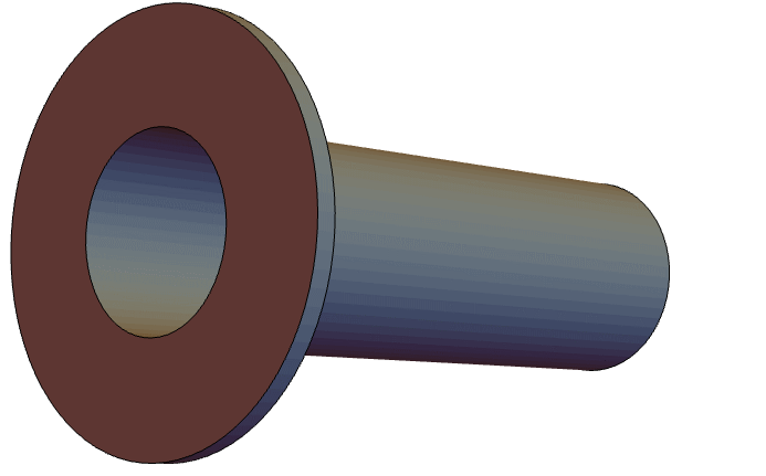
由于管道的几何形状和边界条件关于
轴是旋转对称的,因此可以使用轴对称模型. 描述声波传播的指导方程是轴对称亥姆霍兹 (Helmholtz) 方程.
vars = {p[r, z], ω, {r, z}};
pars = <|"MassDensity" -> Subscript[ρ, air], "SoundSpeed" -> Subscript[c, air], Subscript[c, air] -> 343, Subscript[ρ, air] -> 1.25, "RegionSymmetry" -> "Axisymmetric"|>;轴对称几何体可以用一个二维矩形近似表示,该矩形代表管道在
平面上的横截面:
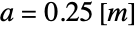
a = 0.25;
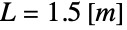
L = 1.5;
Ω = Polygon[{{0, -L}, {a, -L}, {a, 0}, {0, 0}}];在模型中,有两个边界条件. 一个是 NeumannValue,表示活塞的加速度
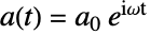
,其中
:
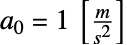
a0 = 1;
Subscript[Τ, acc] = NeumannValue[a0, z == -L];第二个边界条件是具有阻抗
的 AcousticImpedanceValue. 阻抗
由以下近似值给出,其中
是波数:
k = ω / Subscript[c, air];
Subscript[Z, end] = Subscript[ρ, air] * Subscript[c, air] * (1 - (2 BesselJ[1, 2 k a]/2 k a) + I((2 StruveH[1, 2 k a]/2 k a)));
Subscript[Γ, i] = AcousticImpedanceValue[z == 0, vars, pars, <|"SpecificAcousticImpedance" -> Subscript[Z, end]|>];pde = AcousticPDEComponent[vars, pars] == Subscript[Τ, acc] + Subscript[Γ, i];用
求解 PDE,其中 MaxCellMeasure 由
定义,分辨率为 12,以获得精确结果:
λ = 2π Subscript[c, air] / ω;
pfun = ParametricNDSolveValue[pde, p, {r, z}∈Ω, {ω}, Method -> {"PDEDiscretization" -> {"FiniteElement", "MeshOptions" -> {"MaxCellMeasure" -> {"Length" -> λ / 12} /. pars}}}];
pfun1000 = pfun[ω] /. {ω -> (2 Pi)1000};Legended[RegionPlot3D[x^2 + y^2 ≤ a^2 && 0 ≤ PlanarAngle[{0, 0} -> {{a, 0}, {x, y}}] ≤ (4 π/3), {x, -a, a}, {y, -a, a}, {z, -L, 0}, ...], BarLegend[...]]相关指南
-
▪
- 声学 PDE 和边界条件 ▪
- 偏微分方程术语
文本
Wolfram Research (2020),AcousticPDEComponent,Wolfram 语言函数,https://reference.wolfram.com/language/ref/AcousticPDEComponent.html (更新于 2023 年).
CMS
Wolfram 语言. 2020. "AcousticPDEComponent." Wolfram 语言与系统参考资料中心. Wolfram Research. 最新版本 2023. https://reference.wolfram.com/language/ref/AcousticPDEComponent.html.
APA
Wolfram 语言. (2020). AcousticPDEComponent. Wolfram 语言与系统参考资料中心. 追溯自 https://reference.wolfram.com/language/ref/AcousticPDEComponent.html 年
BibTeX
@misc{reference.wolfram_2026_acousticpdecomponent, author="Wolfram Research", title="{AcousticPDEComponent}", year="2023", howpublished="\url{https://reference.wolfram.com/language/ref/AcousticPDEComponent.html}", note=[Accessed: 18-August-2026]}
BibLaTeX
@online{reference.wolfram_2026_acousticpdecomponent, organization={Wolfram Research}, title={AcousticPDEComponent}, year={2023}, url={https://reference.wolfram.com/language/ref/AcousticPDEComponent.html}, note=[Accessed: 18-August-2026]}