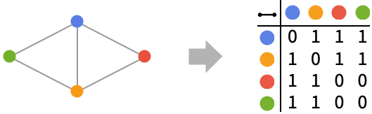
给出图 g 的顶点–顶点邻接矩阵.
AdjacencyMatrix[{vw,…}]
使用 vw 规则来指定 g.
AdjacencyMatrix
给出图 g 的顶点–顶点邻接矩阵.
AdjacencyMatrix[{vw,…}]
使用 vw 规则来指定 g.
更多信息
- 邻接矩阵也被称作连通性矩阵.
- AdjacencyMatrix 返回一个 SparseArray 对象,可以使用 Normal 把它转化成一个普通矩阵.
- 邻接矩阵的元素 aij 是从顶点 νi 到顶点 νj 的有向边的数目.
- 对角线元素 aii 计算顶点 vi 的自环数目.
- 一个无向边被解释为具有相反方向的两条有向边.
- 假设顶点 vi 遵循 VertexList[g] 给出的顺序.
- 一个图的邻接矩阵具有维度
×
,其中
是顶点数.
背景
- AdjacencyMatrix 返回一个被称为邻接矩阵的方阵,其行和列对应于图的顶点而其中的元素 aij 是非负整数,标明的是从顶点 vi 到顶点 vj 的(有向)边的数目. 邻接矩阵给出了图的一种有用的表示方式:可以通过对矩阵的简单操作而计算很多图的性质. 可在给定邻接矩阵上有效进行的图的计算包括顶点度数、入度和出度、顶点间最多
步的路径数目、图的矩阵谱和许多其它性质. - 对有
个顶点的图,邻接矩阵的大小为
×
. 无向图的邻接矩阵是对称的. 对有限简单图(即无向且未加权的,既没有自环也没有多重边的图),对角线元素必须全为 0 且若
与
相邻则其矩阵元素
否则
. - 图的基于特定顶点顺序的显式邻接矩阵表示是唯一的. 然而,由于图的顶点可以打乱排列顺序,所以存在一类邻接矩阵,表示对应的同一同构类的图. 尽管如此,图的同构类的邻接矩阵在模以矩阵行列排列(恰好对应于对图顶点的重命名)的意义下是唯一的.
- AdjacencyGraph 可被用于从邻接矩阵构建图. IncidenceMatrix 给出了图的另一种矩阵表示,用顶点与边的关系代替顶点与顶点的关系. AdjacencyMatrix 并不考虑图的权重,所以计算有边权的图的邻接矩阵时必须使用 WeightedAdjacencyMatrix.
范例
打开所有单元 关闭所有单元基本范例 (2)
范围 (5)
Graph[{12, 13, 23, 24, 34}]AdjacencyMatrix[%]//MatrixFormGraph[{12, 21, 31, 32, 41, 42}]AdjacencyMatrix[%]//MatrixFormAdjacencyMatrix[{1 -> 2, 2 -> 1, 3 -> 1, 3 -> 2, 4 -> 1, 4 -> 2}]//MatrixForm{Graph[{12, 23, 31, 22}], Graph[{11, 12, 23, 31}]}MatrixForm /@ AdjacencyMatrix /@ %AdjacencyMatrix 可用于大规模图:
Graph[Table[iMod[i ^ 2, 10 ^ 3], {i, 0, 10 ^ 3 - 1}]];Timing[m = AdjacencyMatrix[%]]使用 MatrixPlot 来对矩阵进行可视化处理:
MatrixPlot[m]应用 (7)
adjacencyDegree[g_ ? UndirectedGraphQ] := With[{a = AdjacencyMatrix[g]}, Total[a] + Diagonal[a]]adjacencyDegree[[image]]VertexDegree[[image]]adjacencyInDegree[g_ ? DirectedGraphQ] := Total[AdjacencyMatrix[g]]adjacencyInDegree[[image]]VertexInDegree[[image]]adjacencyOutDegree[g_ ? DirectedGraphQ] := Total[AdjacencyMatrix[g]]adjacencyOutDegree[[image]]VertexOutDegree[[image]]graphPathCountMatrix[g_ ? DirectedGraphQ, k_Integer ? Positive] :=
MatrixPower[AdjacencyMatrix[g], k]graphPathCountMatrix[[image], 2]//MatrixFormgraphPathCount[g_ ? DirectedGraphQ, s_, t_, k_Integer ? Positive] :=
MatrixPower[AdjacencyMatrix[g], k][[VertexIndex[g, s], VertexIndex[g, t]]]graphPathCount[[image], 1, 5, 2]计算共被引矩阵,其中两个顶点的共被引数是共同的先驱节点的数目:
cocitationMatrix[g_ ? DirectedGraphQ] := With[{a = AdjacencyMatrix[g]}, a.a - DiagonalMatrix[Diagonal[a.a]]]g = [image];cocitationMatrix[g]//MatrixForm%[[VertexIndex[g, Subscript[J, 2]], VertexIndex[g, Subscript[J, 3]]]]计算耦合矩阵,其中两个顶点之间的耦合是共同的后继节点的数目:
couplingMatrix[g_ ? DirectedGraphQ] := With[{a = AdjacencyMatrix[g]}, a.a - DiagonalMatrix[Diagonal[a.a]]]g = [image];couplingMatrix[g]//MatrixForm%[[VertexIndex[g, Subscript[P, 1]], VertexIndex[g, Subscript[P, 4]]]]属性和关系 (14)
邻接矩阵的行和列遵循由 VertexList 给出的顺序:
g = Graph[{23, 31, 12, 14}, VertexShapeFunction -> "Name", VertexStyle -> Blue]VertexList[g]TableForm[Normal@AdjacencyMatrix[g], TableHeadings -> {c = Style[#, Blue]& /@ %, c}]利用 VertexIndex 求与顶点对相对应的矩阵的行和列:
g = Graph[{23, 31, 12, 14}, VertexShapeFunction -> "Name"](a = AdjacencyMatrix[g])//MatrixForma[[VertexIndex[g, 1], VertexIndex[g, 4]]] == 1与 EdgeQ 相比较:
% == EdgeQ[g, 14]g = CompleteGraph[4]AdjacencyMatrix[g]//MatrixFormSymmetricMatrixQ[%]利用 AdjacencyGraph 从邻接矩阵构建一个图:
AdjacencyGraph[{{0, 1, 0}, {0, 0, 1}, {1, 1, 0}}]AdjacencyMatrix[%]//NormalGridGraph[{2, 3}]Diagonal[AdjacencyMatrix[%]]//Normalg = CompleteGraph[5]Dimensions[AdjacencyMatrix[g]]VertexCount[g]{g, h} = {PetersenGraph[4, 1], HypercubeGraph[3]}IsomorphicGraphQ[g, h]AdjacencyMatrix[g] == AdjacencyMatrix[h]perm = Values[First[FindGraphIsomorphism[g, h]]]AdjacencyMatrix[g][[perm, perm]] == AdjacencyMatrix[h]一个 d 正则图 g 是连通的,当且仅当它的 d 特征值的重数为1:
g = HypercubeGraph[3]VertexDegree[g]Count[Eigenvalues[AdjacencyMatrix[g]], 3]ConnectedGraphQ[g]AdjacencyMatrix[CompleteGraph[10]]//MatrixPlotAdjacencyMatrix[CompleteGraph[{2, 3, 4}]]//MatrixPlotTuranGraph 是二部图:
BipartiteGraphQ[g = TuranGraph[5, 2]]MatrixPlot[AdjacencyMatrix[g]]StarGraph 只在第一列和第一行有1:
AdjacencyMatrix@StarGraph[10]//MatrixPlotPathGraph[Range[20]]MatrixPlot[AdjacencyMatrix[%]]一个线图的邻接矩阵可以通过它的 IncidenceMatrix 计算:
g = GridGraph[{2, 3}]m = IncidenceMatrix[g];MatrixPlot /@ {Transpose[m].m - 2IdentityMatrix[EdgeCount[g]], AdjacencyMatrix[LineGraph[g]]}相关链接
文本
Wolfram Research (2010),AdjacencyMatrix,Wolfram 语言函数,https://reference.wolfram.com/language/ref/AdjacencyMatrix.html (更新于 2015 年).
CMS
Wolfram 语言. 2010. "AdjacencyMatrix." Wolfram 语言与系统参考资料中心. Wolfram Research. 最新版本 2015. https://reference.wolfram.com/language/ref/AdjacencyMatrix.html.
APA
Wolfram 语言. (2010). AdjacencyMatrix. Wolfram 语言与系统参考资料中心. 追溯自 https://reference.wolfram.com/language/ref/AdjacencyMatrix.html 年
BibTeX
@misc{reference.wolfram_2026_adjacencymatrix, author="Wolfram Research", title="{AdjacencyMatrix}", year="2015", howpublished="\url{https://reference.wolfram.com/language/ref/AdjacencyMatrix.html}", note=[Accessed: 11-September-2026]}
BibLaTeX
@online{reference.wolfram_2026_adjacencymatrix, organization={Wolfram Research}, title={AdjacencyMatrix}, year={2015}, url={https://reference.wolfram.com/language/ref/AdjacencyMatrix.html}, note=[Accessed: 11-September-2026]}