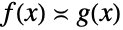
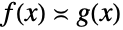
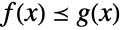
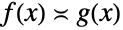
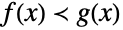
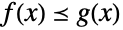
AsymptoticLessEqual[f,g,xx*]
xx*のときに 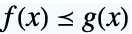 または
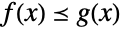
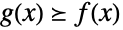
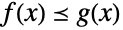
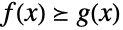
または  となる条件を与える.
AsymptoticLessEqual[f,g,{x1,…,xn}{ ,…,
,…, }]
}]
{x1,…,xn}{ ,…,
,…, }のときに
}のときに  または
または  となる条件を与える.


AsymptoticLessEqual
AsymptoticLessEqual[f,g,xx*]
xx*のときに 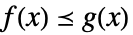 または
または 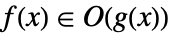 となる条件を与える.
AsymptoticLessEqual[f,g,{x1,…,xn}{ ,…,
,…, }]
}]
{x1,…,xn}{ ,…,
,…, }のときに
}のときに  または
または  となる条件を与える.
詳細とオプション
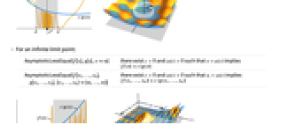
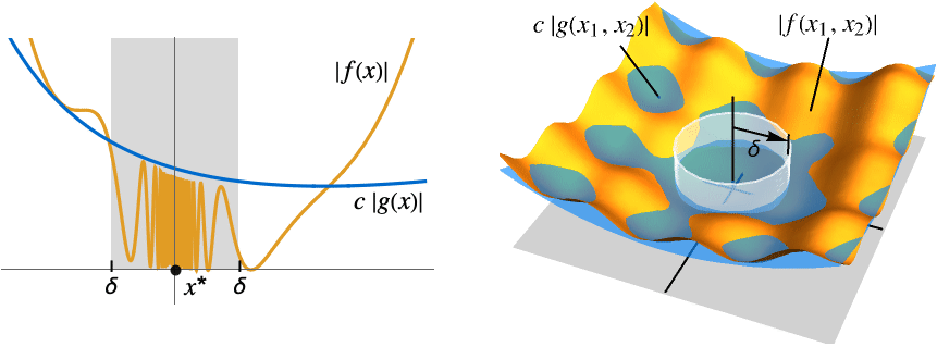
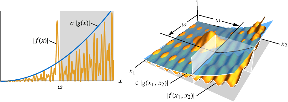
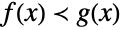
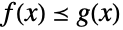
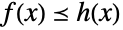
- 「漸近的に以下」は,f が g のbig-oである,f の上限は g である,f の次数は最大でも g である,f は最高で g と同速さで大きくなる等と表現される.点 x*はコンテキストから推測されることが多い.
- 「漸近的に以下」は順序関係で,
 である定数について x が x*の近くにあるときに
![TemplateBox[{{f, (, x, )}}, Abs]<=c TemplateBox[{{g, (, x, )}}, Abs]](Files/AsymptoticLessEqual.ja/10.png "TemplateBox[{{f, (, x, )}}, Abs]<=c TemplateBox[{{g, (, x, )}}, Abs]") であることを意味する.
であることを意味する. - 点の近くの関数や級数の単純な上限を表すために,また,方程式の解や複雑な計算の単純な上限を表すためにしばしば使われる.
- 有限極限点の x*および{
 ,…,
,…, }については以下のようになる.
 -
AsymptoticLessEqual[f[x],g[x],xx*] ![0<TemplateBox[{{x, -, {x, ^, *}}}, Abs]<delta(c,x^*)](Files/AsymptoticLessEqual.ja/13.png "0<TemplateBox[{{x, -, {x, ^, *}}}, Abs]<delta(c,x^*)") が
が![TemplateBox[{{f, (, x, )}}, Abs]<=c TemplateBox[{{g, (, x, )}}, Abs]](Files/AsymptoticLessEqual.ja/14.png "TemplateBox[{{f, (, x, )}}, Abs]<=c TemplateBox[{{g, (, x, )}}, Abs]") を意味する
を意味する  と
と 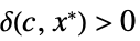 が存在する
が存在するAsymptoticLessEqual[f[x1,…,xn],g[x1,…,xn],{x1,…,xn}{  ,…,
,…, }]
}]![0<TemplateBox[{{{, {{{x, _, 1}, -, {x, _, 1, ^, *}}, ,, ..., ,, {{x, _, n}, -, {x, _, n, ^, *}}}, }}}, Norm]<delta(c,x^*)](Files/AsymptoticLessEqual.ja/19.png "0<TemplateBox[{{{, {{{x, _, 1}, -, {x, _, 1, ^, *}}, ,, ..., ,, {{x, _, n}, -, {x, _, n, ^, *}}}, }}}, Norm]<delta(c,x^*)") が
が![TemplateBox[{{f, (, {{x, _, 1}, ,, ..., ,, {x, _, n}}, )}}, Abs]<=c TemplateBox[{{g, (, {{x, _, 1}, ,, ..., ,, {x, _, n}}, )}}, Abs]](Files/AsymptoticLessEqual.ja/20.png "TemplateBox[{{f, (, {{x, _, 1}, ,, ..., ,, {x, _, n}}, )}}, Abs]<=c TemplateBox[{{g, (, {{x, _, 1}, ,, ..., ,, {x, _, n}}, )}}, Abs]") を意味するな
を意味するな  と
と 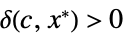 が存在する
が存在する - 無限極限点については以下のようになる.
-
AsymptoticLessEqual[f[x],g[x],x∞]  が
が![TemplateBox[{{f, (, x, )}}, Abs]<=c TemplateBox[{{g, (, x, )}}, Abs]](Files/AsymptoticLessEqual.ja/25.png "TemplateBox[{{f, (, x, )}}, Abs]<=c TemplateBox[{{g, (, x, )}}, Abs]") を意味する
を意味する  と
と  が存在する
が存在するAsymptoticLessEqual[f[x1,…,xn],g[x1,…,xn],{x1,…,xn}{∞,…,∞}] 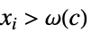 が
が![TemplateBox[{{f, (, {{x, _, 1}, ,, ..., ,, {x, _, n}}, )}}, Abs]<=c TemplateBox[{{g, (, {{x, _, 1}, ,, ..., ,, {x, _, n}}, )}}, Abs]](Files/AsymptoticLessEqual.ja/29.png "TemplateBox[{{f, (, {{x, _, 1}, ,, ..., ,, {x, _, n}}, )}}, Abs]<=c TemplateBox[{{g, (, {{x, _, 1}, ,, ..., ,, {x, _, n}}, )}}, Abs]") を意味する
を意味する  と
と  が存在する
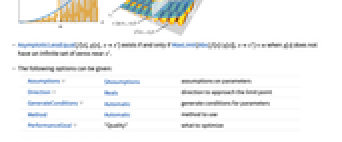
が存在する - g[x]が x*付近に0の無限集合を持たない場合,AsymptoticLessEqual[f[x],g[x],xx*]はMaxLimit[Abs[f[x]/g[x]],xx*]<∞のときかつそのときに限り存在する.
- 次は,使用可能なオプションである.
-
Assumptions $Assumptions パラメータについての仮定 Direction Reals 極限点に近付く方向 GenerateConditions Automatic パラメータについての条件を生成する Method Automatic 使用するメソッド PerformanceGoal "Quality" 何を最適化するか - 次は,Directionの可能な設定である.
-
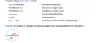
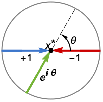
Reals または "TwoSided" 両実数方向から "FromAbove" または -1 上,つまり大きい値から "FromBelow" または +1 下,つまりは小さい値から Complexes すべての複素方向から Exp[ θ]  の方向
の方向{dir1,…,dirn} 変数 xiに方向 diriを使う - x*におけるDirectionExp[ θ]は,曲線の接線が極限点 x*に近付く方向を示す.
- 次は,GenerateConditionsの可能な設定である.
-
Automatic 一般的ではない条件のみ True すべての条件 False 条件なし None 条件が必要な場合には未評価で返す - PerformanceGoalの可能な設定には,$PerformanceGoal,"Quality","Speed"がある."Quality"設定のとき,Limitはより多くの問題を解いたりより簡単な結果を与えたりすることが多いが,より多くの時間とメモリが必要になる可能性がある.
例題
すべて開く すべて閉じる

スコープ (9)


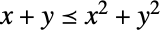
![x^2 TemplateBox[{{x}}, UnitStepSeq]](Files/AsymptoticLessEqual.ja/42.png "x^2 TemplateBox[{{x}}, UnitStepSeq]")

オプション (10)
Assumptions (1)
Assumptionsを使ってパラメータについての条件を指定する:
Direction (5)
GenerateConditions (3)
デフォルトで,特殊な値でしか結果が無効にならない場合は,条件は生成されない:
GenerateConditions->Trueのときは,これらの一般的ではない条件も報告される:
PerformanceGoal (1)
PerformanceGoalを使って潜在的に高価な計算を回避する:
アプリケーション (10)
基本的なアプリケーション (4)




計算の複雑性 (4)
単純なソートアルゴリズム(バブルソート,挿入ソート)は n 個のオブジェクトをソートするのに約 a n2ステップを要する.これに対し,最適化された一般的アルゴリズム(ヒープソート,マージソート)はソートを行うのに約 b n Log[n]のステップを要する.大量のオブジェクトに対しては,最適化されたアルゴリズムの方がソート時間が長くなることは決してない,つまり  であることを示す:
ある種の特別なアルゴリズム(分布数え上げソート,基数ソート)は,考えられる入力についての情報が事前に分かっているので,c n 時間で実行することができる. であることを示す:
バブルソートでは,隣接近傍が比較され,順序が狂っている場合には入れ替えられる.1回のパス(n-1 回の比較)の後で最大要素が末尾になる.このプロセスが残りの n-1個の要素に対して行われ,先頭の2つの要素が残るまでこれが繰り返される.比較と入替えが c ステップだとすると,ソートのステップ総数は次のようになる:


したがって, であり,このアルゴリズムのランタイムは2次であると言われる:
マージソートでは,要素のリストが2つに分割され,半分ずつソートされ,最後に2つの部分が結合される.であるから,ソート時間T[n]は中間を計算する一定の時間 b,各半分を計算する時間2T[n/2],2つの半分を結合するための要素数の倍数 a n の合計になる:
再帰方程式を解いて n 個の要素をソートする時間 t を求める:


したがって  であり,このアルゴリズムのランタイムは
  であると言われる:
巡回セールスマン問題(TSP)は  個の都市を繋ぐ最短経路を求めるものである.馬鹿正直なアルゴリズムは
  通りの経路すべてを試そうとする.Held–Karpアルゴリズムは,それよりも効率よく約
  ステップに短縮する.
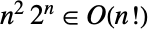 であることを示す:
どちらのアルゴリズムも巡回セールスマン問題の複雑性クラスは,時間 で解ける問題のEXPTIMEと同じくらいであることを示している.Held–Karpアルゴリズムは,
 の
の 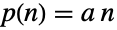 を使うだけで十分である:
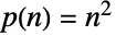
解の近似は  回で求まるので,巡回セールスマン問題の近似は多項式時間で可解な問題の複雑性クラスPに属する.どの多項式アルゴリズムも指数アルゴリズムより速い.つまり
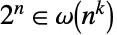 である:
である:
収束判定法 (2)
![sum_(n=1)^inftyTemplateBox[{{a, _, n}}, Abs]<infty](Files/AsymptoticLessEqual.ja/67.png "sum_(n=1)^inftyTemplateBox[{{a, _, n}}, Abs]<infty") であれば,列
であれば,列  は絶対加算可能であると言われる.第2列が
  なら,比較判定法は,
 が絶対加算可能なら
  も絶対加算可能であると述べる.この判定法を使って,
 の総和と比較することによって
  が収束することを示す:
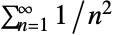
SumConvergenceが与える答と比較する:
 と比較可能な別の列に
 ![TemplateBox[{n}, PrimePi]/(n^3log(n))](Files/AsymptoticLessEqual.ja/76.png "TemplateBox[{n}, PrimePi]/(n^3log(n))") がある.したがって,これも絶対加算可能である:
がある.したがって,これも絶対加算可能である:


![int_a^bTemplateBox[{{f, , {(, x, )}}}, Abs]dx<infty](Files/AsymptoticLessEqual.ja/79.png "int_a^bTemplateBox[{{f, , {(, x, )}}}, Abs]dx<infty") なら,関数
なら,関数  は
は で完全に積分可能であると言われる.
 と
と  が開区間
が開区間 で連続であり,
 と
と  の両方で
の両方で  なら,比較判定法は
  が完全に積分可能なら
  もそうであるとする.この判定法を使って
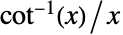 が
が で完全に積分可能であることを示す:



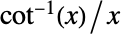


 と
と  の両方で
の両方で  ,したがって
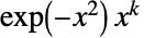 の絶対的積分可能性は次のようになる:






特性と関係 (8)
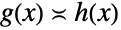
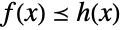
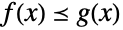
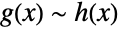
AsymptoticLessEqualは反射的ではない.つまり,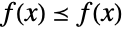 である:
である:
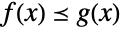
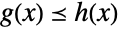
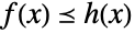
しかし,対称関係ではない.つまり,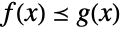 であるから
であるから 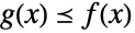 であるということにはならない:
MaxLimit[Abs[f[x]/g[x]],xx0]<∞のときかつそのときに限りAsymptoticLessEqual[f[x],g[x],xx0]である:
Limit[Abs[f[x]/g[x]],xx0]<∞であればAsymptoticLessEqual[f[x],g[x],xx0]である:
しかし,極限がIndeterminateのときは不確定である:
テキスト
Wolfram Research (2018), AsymptoticLessEqual, Wolfram言語関数, https://reference.wolfram.com/language/ref/AsymptoticLessEqual.html.
CMS
Wolfram Language. 2018. "AsymptoticLessEqual." Wolfram Language & System Documentation Center. Wolfram Research. https://reference.wolfram.com/language/ref/AsymptoticLessEqual.html.
APA
Wolfram Language. (2018). AsymptoticLessEqual. Wolfram Language & System Documentation Center. Retrieved from https://reference.wolfram.com/language/ref/AsymptoticLessEqual.html