

AsymptoticSolve
AsymptoticSolve[eqn,yb,x->a]
computes asymptotic approximations of solutions y[x] of the equation eqn passing through {a,b}.
AsymptoticSolve[eqn,{y},x->a]
computes asymptotic approximations of solutions y[x] of the equation eqn for x near a.
AsymptoticSolve[eqns,{y1,y2,…}{b1,b2,…},{x1,x2,…}{a1,a2,…}]
computes asymptotic approximations of solutions {y1[x1,x2,…],y2[x1,x2,…],…} of the system of equations eqns.
AsymptoticSolve[eqns,…,{{x1,x2,…},{a1,a2,…},n}]
computes the asymptotic approximation to order n.
computes only solutions that are real valued for real argument values.
Details and Options
- Asymptotic approximations are typically used to solve problems for which no exact solution can be found or to get simpler answers for computation, comparison and interpretation.
- AsymptoticSolve[eqn,…,xa] computes the leading term in an asymptotic expansion for eqn. Use SeriesTermGoal to specify more terms.
- The asymptotic approximation yn[x] is often given as a sum yn[x]
 αkϕk[x], where {ϕ1[x],…,ϕn[x]} is an asymptotic scale ϕ1[x]≻ϕ2[x]≻⋯>ϕn[x] as xa. Then the result satisfies AsymptoticLess[y[x]-yn[x],ϕn[x],xa] or y[x]-yn[x]∈o[ϕn[x]] as xa.
 - Common asymptotic scales include:
-

Taylor scale when xa 
Laurent scale when xa 
Laurent scale when x±∞ 
Puiseux scale when xa - The scales used to express the asymptotic approximation are automatically inferred from the problem and can often include more exotic scales.
- The center coordinates a and b can be any finite or infinite real or complex numbers.
- The order n must be a positive integer and specifies order of approximation for the asymptotic solution. It may not be related to polynomial degree.
- The system of equations eqns can be any logical combination of equations.
- The following options can be given:
-
Assumptions $Assumptions assumptions to make about parameters Direction Automatic direction in which x approaches a GenerateConditions Automatic whether to generate answers that involve conditions on parameters Method Automatic method to use PerformanceGoal $PerformanceGoal aspects of performance to optimize SeriesTermGoal Automatic number of terms in the approximation - Possible settings for Direction include:
-
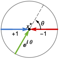
Reals or "TwoSided" from both real directions "FromAbove" or -1 from above or larger values "FromBelow" or +1 from below or smaller values Complexes from all complex directions Exp[ θ] in the direction 
{dir1,…,dirn} use direction diri for variable xi independently - DirectionExp[ θ] at x* indicates the direction tangent of a curve approaching the limit point x*.
- For finite values of a, the Automatic setting means from above.
- When domain Reals is specified, the solutions are real valued when x approaches a in the indicated Direction.
- Possible settings for GenerateConditions include:
-
Automatic nongeneric conditions only True all conditions False no conditions None return unevaluated if conditions are needed - Possible settings for PerformanceGoal include $PerformanceGoal, "Quality" and "Speed". With the "Quality" setting, AsymptoticSolve typically solves more problems or produces simpler results, but it potentially uses more time and memory.
Examples
open all close allBasic Examples (5)
Find asymptotic approximations of solutions passing through the point {0,0}:
AsymptoticSolve[E^y - Cos[x y] + x == 0, {y, 0}, {x, 0, 7}]Find asymptotic approximations of solutions for x near 0:
AsymptoticSolve[x y^4 - (x + 1) y^2 + x == 1, {y}, {x, 0, 3}]Find the leading terms of asymptotic approximations of solutions as ![]() :
:
AsymptoticSolve[y ^ 3 + E ^ x y + x Log[x] == 0, y, x -> Infinity]Find only the solutions that are real valued when x approaches 0 from above:
AsymptoticSolve[x y^4 - (x + 1) y^2 + x == 1, {y}, {x, 0, 3}, Reals]Find asymptotic approximations of solutions of a system of equations:
AsymptoticSolve[x^2 - u (y + 1) == y^2 - v (x + 1) && u^2 - u (x + 1) == v^2 + v (y + 1), {{u, v}, {0, 0}}, {{x, y}, {0, 0}, 3}]Scope (18)
One-Dimensional Solutions in 2D (8)
Power series solutions of polynomial equations passing through a specified point:
AsymptoticSolve[y ^ 3 - x y == 24, {y, 3}, {x, 1, 3}]Plot the asymptotic solution and the solution it approximates:
asympt = First[y /. %];
exact[x_] := Last[y /. NSolve[y ^ 3 - x y == 24, y, Reals]]Plot[{asympt, exact[x]}, {x, -50, 50}, PlotStyle -> {Dashed, DotDashed}]Power series solutions of analytic equations passing through a specified point:
f = Erf[x + y] - Log[1 + Sin[x y]];AsymptoticSolve[f == 0, {y, 0}, {x, 0, 3}]Plot the asymptotic solution and the solution it approximates:
asympt = First[y /. %];
exact[x_] := y /. FindRoot[f, {y, asympt}]Plot[{asympt, exact[x]}, {x, -0.4, 0.4}, PlotStyle -> {Dashed, DotDashed}]Puiseux series solutions of polynomial equations passing through a specified point:
AsymptoticSolve[y ^ 5 - x y + x ^ 2 == 0, {y, 0}, {x, 0, 5}]Solutions that are real valued when x approaches 0 from above:
AsymptoticSolve[y ^ 5 - x y + x ^ 2 == 0, {y, 0}, {x, 0, 5}, Reals]Solutions that are real valued when x approaches 0 from below:
AsymptoticSolve[y ^ 5 - x y + x ^ 2 == 0, {y, 0}, {x, 0, 5}, Reals, Direction -> "FromBelow"]Puiseux series solutions of analytic equations passing through a specified point:
AsymptoticSolve[Sin[x y] - y ^ 2 + x == 0, {y, 0}, {x, 0, 5}]Asymptotic series solutions passing through a specified point:
AsymptoticSolve[Sin[y] - y ^ 2 + Cos[y] / Log[x] == 0, {y, 0}, {x, 0, 5}]Solutions of polynomial equations near a specified value of the independent variable:
AsymptoticSolve[x y ^ 4 + y ^ 2 - x ^ 2 y == 1, {y}, {x, 0, 3}]Real asymptotic series solutions at infinity:
f = y ^ 5 - y / Sqrt[x] + x Log[x];AsymptoticSolve[f == 0, {y}, {x, Infinity, 3}, Reals]Plot the asymptotic solution and the solution it approximates:
asympt = First[y /. %];
exact[x_] := First[y /. NSolve[f == 0, y, Reals]]Plot[{asympt, exact[x]}, {x, 1, 5}, PlotStyle -> {Dashed, DotDashed}]Equations with symbolic parameters:
AsymptoticSolve[Sin[x y] - y Log[a + y] + x == 0, {y, 0}, {x, 0, 3}]Conditions on parameters may be generated:
AsymptoticSolve[y ^ 4 + a y ^ 3 + a x y - x ^ 2 + a x ^ 2 == 0, {y, Root[# ^ 4 + a # ^ 3&, 1]}, {x, 0, 3}]One-Dimensional Solutions in nD (5)
Power series solutions of polynomial systems passing through a specified point:
eqns = y ^ 3 - t x y == 21 && x ^ 2 - t ^ 2 y == 1;AsymptoticSolve[eqns, {{x, y}, {2, 3}}, {t, 1, 3}]Plot the asymptotic solution and the solution it approximates:
asympt = First[{t, x, y} /. %];
exact = {t, x, y} /. Solve[eqns, {x, y}, Reals][[2]];ParametricPlot3D[{asympt, exact}, {t, 0, 2}, PlotStyle -> {Dashed, DotDashed}]Power series solutions of analytic systems passing through a specified point:
eqns = Sin[t + x] + Cos[y] == t + 1 && Log[1 + x + y] - Sin[t] == 0;AsymptoticSolve[eqns, {{x, y}, {0, 0}}, {t, 0, 5}]Plot the asymptotic solution and the solution it approximates:
asympt = First[{t, x, y} /. %];
exact[t_] := {t, x, y} /. FindRoot[eqns, {{x, asympt[[2]]}, {y, asympt[[3]]}}]ParametricPlot3D[{asympt, exact[t]}, {t, -0.9, 0.9}, PlotStyle -> {Dashed, DotDashed}]Puiseux series solutions of polynomial systems passing through a specified point:
AsymptoticSolve[y ^ 2 - t x + t == 0 && x ^ 2 + t y == 0, {{x, y}, {0, 0}}, {t, 0, 2}]None of the solutions are real valued when t approaches 0 from above:
AsymptoticSolve[y ^ 2 - t x + t == 0 && x ^ 2 + t y == 0, {{x, y}, {0, 0}}, {t, 0, 2}, Reals]Two of the solutions are real valued when t approaches 0 from below:
AsymptoticSolve[y ^ 2 - t x + t == 0 && x ^ 2 + t y == 0, {{x, y}, {0, 0}}, {t, 0, 2}, Reals, Direction -> "FromBelow"]Solutions of polynomial systems near a specified value of the independent variable:
AsymptoticSolve[y ^ 3 - t x y == 0 && x ^ 2 - t ^ 2 y == 1, {{x, y}}, {t, 0, 3}]Equations with symbolic parameters:
AsymptoticSolve[{Sin[t + a x] + Cos[y] == t + 1, Log[1 + x + y] - Sin[t] == 0}, {{x, y}, {0, 0}}, {t, 0, 5}]Higher-Dimensional Solutions in nD (5)
Power series solutions of polynomial equations passing through a specified point:
AsymptoticSolve[z ^ 5 - 2z ^ 3 + 2z + x ^ 2 - y == 0, {z, 0}, {{x, y}, {0, 0}, 5}]Plot the asymptotic solution and the solution it approximates:
asympt = First[z /. %];
exact[x_, y_] := First[z /. NSolve[z ^ 5 - 2z ^ 3 + 2z + x ^ 2 - y == 0, z, Reals]];Plot3D[{asympt, exact[x, y]}, {x, -1, 1}, {y, -1, 1}, PlotLegends -> {"Asymptotic", "Exact"}, PlotStyle -> Opacity[0.7], BoxRatios -> 1]Power series solutions of analytic equations passing through a specified point:
AsymptoticSolve[Exp[z + x - y] - Cos[x y] + x - y == 0, {z, 0}, {{x, y}, {0, 0}, 3}]Plot the asymptotic solution and the solution it approximates:
asympt = First[z /. %];
exact[x_, y_] := z /. FindRoot[Exp[z + x - y] - Cos[x y] + x - y == 0, {z, asympt}]Plot3D[{asympt, exact[x, y]}, {x, -1, 1}, {y, -1, 1}, PlotLegends -> {"Asymptotic", "Exact"}, PlotStyle -> Opacity[0.7], BoxRatios -> 1]Power series solutions of polynomial systems passing through a specified point:
AsymptoticSolve[x ^ 2 - u (y + 1) == y ^ 2 - v (x + 1) + w && u ^ 2 - u (x + 1) == v ^ 2 + v (y + 1) - w && x + y == u + v + w, {{u, v, w}, {0, 0, 0}}, {{x, y}, {0, 0}, 3}]Power series solutions of analytic systems passing through a specified point:
AsymptoticSolve[{Sin[u + x] + Cos[y] == v + 1, Log[1 + x + y] - u - Sin[u v] == 0}, {{u, v}, {0, 0}}, {{x, y}, {0, 0}, 3}]Power series solutions of polynomial systems near specified values of independent variables:
AsymptoticSolve[x ^ 2 - u == y ^ 2 - v(x + 1) - u ^ 2 && u ^ 2 - u(x + 1) == v ^ 2 + v, {{u, v}}, {{x, y}, {0, 0}, 2}]Options (9)
Assumptions (1)
Specify conditions on parameters using Assumptions:
AsymptoticSolve[y ^ 3 - a y + x ^ 2y + x == 0, {y}, {x, 0, 3}, Reals, Assumptions -> a > 0]Different assumptions can produce different results:
AsymptoticSolve[y ^ 3 - a y + x ^ 2y + x == 0, {y}, {x, 0, 3}, Reals, Assumptions -> a < 0]Direction (3)
By default, AsymptoticSolve gives solutions valid when x approaches 0 from above:
AsymptoticSolve[y ^ 3 + x ^ 2y + x == 0, {y}, {x, 0, 3}, Reals]This finds the solutions valid when x approaches 0 from below:
AsymptoticSolve[y ^ 3 + x ^ 2y + x == 0, {y}, {x, 0, 3}, Reals, Direction -> "FromBelow"]Complex solutions may also depend on the direction:
AsymptoticSolve[y ^ 2 + E ^ (-2 / x) y + E ^ (-1 / x) == 0, {y, 0}, {x, 0, 5}, Direction -> "FromAbove"]AsymptoticSolve[y ^ 2 + E ^ (-2 / x) y + E ^ (-1 / x) == 0, {y, 0}, {x, 0, 5}, Direction -> "FromBelow"]This gives solutions that are real when x approaches 0 from a complex direction:
AsymptoticSolve[x y ^ 7 + 2 x ^ 4 y ^ 6 + 3 x ^ 4 y ^ 3 - 2 x ^ 7 y ^ 2 - x ^ 10 == 0, {y, 0}, {x, 0, 3}, Reals, Direction -> E ^ (2 I Pi / 3)]GenerateConditions (3)
By default, AsymptoticSolve gives conditions it assumed to obtain the result:
AsymptoticSolve[y ^ 3 + a y ^ 2 - x == 0, {y}, {x, 0, 3}, Reals]This gives the result without the assumed conditions:
AsymptoticSolve[y ^ 3 + a y ^ 2 - x == 0, {y}, {x, 0, 3}, Reals, GenerateConditions -> False]By default, assumed conditions that are generically true are not reported:
AsymptoticSolve[y ^ 3 + a y ^ 2 - x == 0, {y}, {x, 0, 2}]With GenerateConditions->True, all conditions are reported:
AsymptoticSolve[y ^ 3 + a y ^ 2 - x == 0, {y}, {x, 0, 2}, GenerateConditions -> True]With GenerateConditions->None, AsymptoticSolve returns only generically valid results:
AsymptoticSolve[y ^ 3 + a y ^ 2 - x == 0, {y}, {x, 0, 2}, GenerateConditions -> None]If nongeneric conditions are needed, AsymptoticSolve returns unevaluated:
AsymptoticSolve[y ^ 3 + a y ^ 2 - x == 0, {y}, {x, 0, 2}, Reals, GenerateConditions -> None]Method (1)
Return a series whenever the result is a power series or a Puiseux series:
AsymptoticSolve[Tan[x + y] ^ 3 - y ^ 2 + x == 0, {y, 0}, {x, 0, 3}, Method -> {"SeriesOutput" -> Automatic}]Check that the series solutions satisfy the equation:
Tan[x + y] ^ 3 - y ^ 2 + x /. %SeriesTermGoal (1)
By default, AsymptoticSolve[eqn,…,xa] computes the leading terms of the solutions:
AsymptoticSolve[Cos[x y] - Exp[y ^ 2 - 2x ^ 2] == 0, y -> 0, x -> 0]Use SeriesTermGoal to obtain more terms:
AsymptoticSolve[Cos[x y] - Exp[y ^ 2 - 2x ^ 2] == 0, y -> 0, x -> 0, SeriesTermGoal -> 5]Applications (12)
Implicit Functions (3)
The equation ![]() implicitly defines two different functions
implicitly defines two different functions ![]() near each
near each ![]() . Compute third-order asymptotic approximations for these two functions near
. Compute third-order asymptotic approximations for these two functions near ![]() :
:
AsymptoticSolve[y^2 == x, y, {x, 4, 3}]Define functions based on these expansions:
{yA1[x_], yA2[x_]} = y /. %;At the point ![]() , these two functions have different values:
, these two functions have different values:
{yA1[4], yA2[4]}However, both exactly satisfy the equation ![]() at
at ![]() :
:
{yA1[4] ^ 2 == 4, yA2[4] ^ 2 == 4}Visualize the equation and the approximations to its two branches:
ContourPlot[{y^2 == x, y == yA1[x], y == yA2[x]}, {x, -1, 6}, {y, -3, 3}, Epilog -> {PointSize[Large], Point[{{4, -2}, {4, 2}}]}]In this case, it is easy to solve exactly for the two implicitly defined functions:
{y1[x_], y2[x_]} = y /. Solve[y ^ 2 == x, y]The two expressions returned by AsymptoticSolve are the series of the exact solutions:
Series[yA1[x] - y1[x], {x, 4, 3}]//NormalSeries[yA2[x] - y2[x], {x, 4, 3}]//NormalCompute the second-order asymptotic approximations to the unit circle ![]() at
at ![]() :
:
{yR1[x_], yR2[x_]} = y /. AsymptoticSolve[y ^ 2 + x ^ 2 == 1, y, {x, 0, 2}]The approximations closely track the circle of both larger and smaller values of ![]() at these regular points:
at these regular points:
ContourPlot[{y ^ 2 + x ^ 2 == 1, y == yR1[x], y == yR2[x]}, {x, -3 / 2, 3 / 2}, {y, -3 / 2, 3 / 2}, Epilog -> {PointSize[Large], Point[{{0, 1}, {0, -1}}]}]At the singular point ![]() , the approximation uses fractional powers:
, the approximation uses fractional powers:
{yS1[x_], yS2[x_]} = y /. AsymptoticSolve[y ^ 2 == 1 - x ^ 2, y, {x, 1, 2}]Visually, the approximations seem to only be defined for values of ![]() :
:
ContourPlot[{y ^ 2 + x ^ 2 == 1, y == yS1[x], y == yS2[x]}, {x, -3 / 2, 3 / 2}, {y, -3 / 2, 3 / 2}, Epilog -> {PointSize[Large], Point[{1, 0}]}]This is because at ![]() the functions switch from being real to purely imaginary:
the functions switch from being real to purely imaginary:
Plot[{Im[yS1[x]], Im[yS2[x]]}, {x, 0, 2}, PlotTheme -> {"Detailed", "DashedLines"}]Trying to find solutions over the reals will therefore fail:
AsymptoticSolve[y ^ 2 + x ^ 2 == 1, y, {x, 1, 2}, Reals]However, it is possible to find purely real expressions if restricting to smaller values of ![]() :
:
AsymptoticSolve[y ^ 2 == 1 - x ^ 2, y, {x, 1, 2}, Reals, Direction -> "FromBelow"]The curve ![]() crosses the line
crosses the line ![]() infinitely many times. On any section that passes the vertical line test—any vertical line intersects the curve only once; no vertical line intersects the section more than once—a function is implicitly defined:
infinitely many times. On any section that passes the vertical line test—any vertical line intersects the curve only once; no vertical line intersects the section more than once—a function is implicitly defined:
ContourPlot[{Sin[y] == x, x == 0}, {x, -1, 1}, {y, -3π, 3π}, PlotTheme -> "DashedLines"]Compute an approximation for the section that goes through the origin:
AsymptoticSolve[Sin[y] == x, {y, 0}, {x, 0, 3}]Note that this matches the Taylor series of ![]() , the inverse function of
, the inverse function of ![]() :
:
Series[ArcSin[x], {x, 0, 3}]Compute an approximation for the section that goes through the point ![]() :
:
AsymptoticSolve[Sin[y] == x, {y, Pi}, {x, 0, 3}]Visualize the curve and the two approximations:
ContourPlot[{Sin[y] == x, x == 0, y == x + (x^3/6), y == π - x - (x^3/6)}, {x, -1.5, 1.5}, {y, -π, 2π}, IconizedObject[«ContourPlot options»]]Perturbed Equations (2)
Find solutions of a perturbed polynomial equation:
f = x ^ 3 - (6 + ϵ)x ^ 2 + (11 + ϵ)x - 6 + ϵ;AsymptoticSolve[f == 0, {x}, {ϵ, 0, 3}]Plot the asymptotic solutions and the solutions they approximate:
asympt = x /. %;
exact = x /. Solve[f == 0, x];Plot[{asympt, exact}, {ϵ, 0, 0.5}, PlotStyle -> {Dashed, DotDashed}]Investigate the behavior of solutions of an analytic equation under a small perturbation:
f = Cos[x] - 1 + ϵ E ^ x;AsymptoticSolve[f == 0, {x, 0}, {ϵ, 0, 3}]Plot the asymptotic solutions and the solutions they approximate:
asympt = x /. %;
exact[s_] := x /. FindRoot[f, {x, s}]Show[Plot[{#, exact[#]}, {ϵ, 0, 0.2}, PlotStyle -> {Dashed, DotDashed}]& /@ asympt, PlotRange -> All]Series Solutions of Equations (2)
Find a series solution of an equation at a nonsingular point:
f = Cos[x + y] - x + y - 1;The derivative of ![]() with respect to
with respect to ![]() does not vanish at
does not vanish at ![]() :
:
D[f, y] /. {x -> 0, y -> 0}Find the series solution up to order five:
AsymptoticSolve[f == 0, {y, 0}, {x, 0, 5}]The result satisfies the equation:
Series[f /. %[[1]], {x, 0, 5}]Find a multivariate series solution of a system of equations at a nonsingular point:
f = Sin[x + y + u + v] - u x + v y;
g = Exp[x - u] + Exp[y - v] - 2 Cos[x - v] + y - u;
The Jacobian of ![]() with respect to
with respect to ![]() does not vanish at
does not vanish at ![]() :
:
Det[D[{f, g}, {{x, y}}]] /. {x -> 0, y -> 0, u -> 0, v -> 0}Find the series solution up to order three:
AsymptoticSolve[f == 0 && g == 0, {{x, y}, {0, 0}}, {{u, v}, {0, 0}, 3}]The result satisfies the equations:
Series[{f, g} /. %[[1]] /. {u -> t u, v -> t v}, {t, 0, 3}]Asymptotic Approximations of Curves (3)
Find Puiseux series solutions in a neighborhood of a singular point of an algebraic plane curve:
f = y ^ 6 - 5x y ^ 4 + 3x ^ 2 y ^ 4 + 10x ^ 3 y ^ 2 + 3x ^ 4 y ^ 2 - x ^ 5 + x ^ 6;ls = AsymptoticSolve[f == 0, {y, 0}, {x, 0, 3}, Reals, Direction -> "FromBelow"]rs = AsymptoticSolve[f == 0, {y, 0}, {x, 0, 3}, Reals, Direction -> "FromAbove"]Plot the asymptotic solutions and the curve they approximate near 0:
lp = ParametricPlot[Evaluate[{x, y} /. ls], {x, -1, 0}, PlotStyle -> {{Red, Dashed}}];rp = ParametricPlot[Evaluate[{x, y} /. rs], {x, 0, 1}, PlotStyle -> {{Red, Dashed}}];exact = ContourPlot[f == 0, {x, -1, 1}, {y, -1, 1}, PlotPoints -> 100];Show[{exact, lp, rp}]Find Puiseux series solutions in a neighborhood of a singular point of an algebraic space curve:
eqns = z ^ 2 - y ^ 2 + x y z + x ^ 2 z + x == 0 && x ^ 2 z ^ 2 + x y ^ 2 + y z + x y + x ^ 2 == 0;ls = AsymptoticSolve[eqns, {{y, z}, {0, 0}}, {x, 0, 3}, Reals, Direction -> "FromBelow"]rs = AsymptoticSolve[eqns, {{y, z}, {0, 0}}, {x, 0, 3}, Reals, Direction -> "FromAbove"]Plot the asymptotic solutions:
lasym = {x, y, z} /. ls;
rasym = {x, y, z} /. rs;
lp = ParametricPlot3D[lasym, {x, -0.3, 0}, PlotStyle -> {{Red, Dashed}}];
rp = ParametricPlot3D[rasym, {x, 0, 0.3}, PlotStyle -> {{Red, Dashed}}];
Find numeric solutions using asymptotic solution values as starting points:
nsol[s_] := {x, y, z} /. FindRoot[eqns, {{y, s[[2]]}, {z, s[[3]]}}]lpn = ParametricPlot3D[nsol /@ lasym, {x, -0.3, 0}, PlotStyle -> Blue];
rpn = ParametricPlot3D[nsol /@ rasym, {x, 0, 0.3}, PlotStyle -> Blue];Compare the numeric solutions and the asymptotic solutions:
Show[{lpn, rpn, lp, rp}, PlotRange -> All, BoxRatios -> 1]Show the curve as an intersection of two surfaces:
surf = ContourPlot3D[Evaluate[List@@eqns], {x, -0.3, 0.3}, {y, -0.6, 0.6}, {z, -0.6, 0.6}, Mesh -> None, ContourStyle -> {Directive[Orange, Opacity[0.3]], Directive[Yellow, Opacity[0.3]]}];Show[{surf, lpn, rpn, lp, rp}, PlotRange -> All, BoxRatios -> 1]Approximate Fermat's spiral near 0:
AsymptoticSolve[x == r Cos[r ^ 2] && y == r Sin[r ^ 2], {{y, r}, {0, 0}}, {x, 0, 12}]asympt = First[y /. %];
ap = Plot[asympt, {x, 0, 1}, PlotStyle -> {Red, DotDashed}];
spiral = ParametricPlot[{r Cos[r ^ 2], r Sin[r ^ 2]}, {r, 0, 5}, PlotStyle -> Dashed];Show[{ap, spiral}, PlotRange -> All, AspectRatio -> Automatic]Asymptotic Solutions of Physics Problems (2)
Solve Kepler's equation for the eccentric anomaly ![]() in terms of the mean anomaly
in terms of the mean anomaly ![]() :
:
AsymptoticSolve[M == Ε - e Sin[Ε], {Ε, 0}, {M, 0, 7}]Compare with the exact solution for eccentricity ![]() :
:
asympt = First[Ε /. %] /. e -> 1 / 2;
exact[M_] := First[Ε /. Solve[M == Ε - 1 / 2Sin[Ε], Ε, Reals]//Quiet]Plot[{asympt, exact[M]}, {M, 0, 0.7}, PlotStyle -> {Dashed, DotDashed}]Study the energy levels of a particle of mass ![]() in a one-dimensional box of width
in a one-dimensional box of width ![]() and depth
and depth ![]() . Solutions
. Solutions ![]() ,
, ![]() and
and ![]() of the time-independent Schrödinger equation to the left of the box, inside the box, and to the right of the box are given by:
of the time-independent Schrödinger equation to the left of the box, inside the box, and to the right of the box are given by:
α = (Sqrt[2 m (V - Ε)]/ℏ);k = (Sqrt[2 m Ε]/ℏ);
Subscript[ψ, 1] = g Exp[α x];Subscript[ψ, 2] = a Sin[k x] + b Cos[k x];Subscript[ψ, 3] = h Exp[-α x];
The solution must be continuously differentiable on the boundary of the box:
bconds = {(Subscript[ψ, 1] /. x -> -L / 2) == (Subscript[ψ, 2] /. x -> -L / 2), (Subscript[ψ, 2] /. x -> L / 2) == (Subscript[ψ, 3] /. x -> L / 2), (Subscript[∂, x]Subscript[ψ, 1] /. x -> -L / 2) == (Subscript[∂, x]Subscript[ψ, 2] /. x -> -L / 2), (Subscript[∂, x]Subscript[ψ, 2] /. x -> L / 2) == (Subscript[∂, x]Subscript[ψ, 3] /. x -> L / 2)}The homogenous linear equations admit nonzero solutions if their coefficient matrix is singular:
eqn = Det[CoefficientArrays[bconds, {a, b, g, h}][[2]]] == 0Assume that ![]() and
and ![]() are 1 and the units are chosen so that
are 1 and the units are chosen so that ![]() :
:
m = 1;L = 1; ℏ = 1;Find the possible energy levels for ![]() :
:
e1 = Ε /. Solve[(eqn /. V -> 1) && Ε > 0, Ε, Reals]Compute the asymptotic solution near ![]() :
:
AsymptoticSolve[eqn, {Ε, N[e1[[1]], 20]}, {V, 1, 5}]Compare the asymptotic solution and the minimum exact solution:
asympt = First[Ε /. %];
exact = Table[{V, Min[Ε /. Solve[eqn && Ε ≥ 1 / 1000, Ε, Reals]]}, {V, 1 / 4, 4, 1 / 4}];Show[{Plot[asympt, {V, 0.25, 4}], ListPlot[exact, PlotStyle -> Red]}]Text
Wolfram Research (2019), AsymptoticSolve, Wolfram Language function, https://reference.wolfram.com/language/ref/AsymptoticSolve.html (updated 2020).
CMS
Wolfram Language. 2019. "AsymptoticSolve." Wolfram Language & System Documentation Center. Wolfram Research. Last Modified 2020. https://reference.wolfram.com/language/ref/AsymptoticSolve.html.
APA
Wolfram Language. (2019). AsymptoticSolve. Wolfram Language & System Documentation Center. Retrieved from https://reference.wolfram.com/language/ref/AsymptoticSolve.html