

Compile
詳細とオプション
- Compileが取り扱うタイプ
-
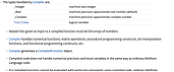
_Integer 機械サイズの整数 _Real 機械精度の近似実数(デフォルト値) _Complex 機械精度の近似複素数 True | False 論理変数 - コンパイルされる関数の入力として与えられるネストしたリストは,数値からなる完全配列でなければならない.
- Compileは,数値関数,行列演算,手続き型プログラミング構文,リスト操作関数,関数型プログラミング構文等に使うことができる.
- Compileは,CompiledFunctionオブジェクトを作成する.
- コンパイルされたコードは,通常のWolfram言語のコードと同様の数値的な精度や局所変数の取扱いをするとは限らない.
- コンパイルされたコードを使った特定の引数でコンパイルされた関数が評価できない場合,代りとして通常のWolfram言語のコードが使用される.
- 通常のWolfram言語のコードを,コンパイルされたコードの中で使用することができる.このWolfram言語コードで得られた結果は,Compileの第3引数で特に指定されない限り近似実数であるとみなされる.
- Compileによってオブジェクトが評価される回数やその順が通常のWolfram言語のコードと異なる場合がある.
- Compileは属性HoldAllを持ち,デフォルトにより,コンパイルされる前に評価を行わない.
- Compile[…,Evaluate[expr]]の設定により,式 expr をコンパイルの前に,シンボル的に評価するように指定できる.
- 使用可能なオプション
-
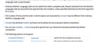
CompilationOptions Automatic コンパイルのプロセスに関するオプション CompilationTarget $CompilationTarget コード生成でターゲットとするランタイム Parallelization Automatic コンパイルされた関数の実行の際の並列制御 RuntimeAttributes {} コンパイルされた関数の評価属性 RuntimeOptions Automatic コンパイルされた関数のランタイムオプション
例題
すべて開く すべて閉じる例 (1)
関数Sin[x]+x^2-1/(1-x)を機械実数 x についてコンパイルする:
cf = Compile[{{x, _Real}}, Sin[x] + x ^ 2 - 1 / (1 + x)]CompiledFunctionは機械数で評価する:
cf[Pi]Plot[cf[x], {x, -1, 1}]スコープ (1)
のニュートン反復を取り,直近の根を見付けるように関数をコンパイルする:
newt = Compile[{{z, _Complex}, {n, _Integer}}, Module[{zn = z},
Do[zn = (2 zn + 1 / zn ^ 2) / 3, {n}];If[Re[zn] > 0, 1, If[Im[zn] > 0, 2, 3]]]]ArrayPlot[Table[newt[x + I y, 25], {y, -1, 1, 2. / 199}, {x, -1, 1, 2. / 199}]]オプション (9)
CompilationOptions (1)
デフォルト設定のAutomaticでは,同じ結果を複数回評価することを避けてより効率的なコードを生成する:
Compile[ {{x}}, x ^ 2 + Sin[x ^ 2]]Compile[ {{x}}, x ^ 2 + Sin[x ^ 2], CompilationOptions -> {"ExpressionOptimization" -> False}]CompilationTarget (2)
c = Compile[ {{x}}, x ^ 2 + Sin[x ^ 2], CompilationTarget -> "C"];
c[ 10.5]これはCコード生成によるスピードアップという利点を示しているより大きい例である:
c = Compile[ {{x, _Real}, {n, _Integer}},
Module[ {sum, inc}, sum = 1.0;inc = 1.0;Do[inc = inc * x / i;sum = sum + inc, {i, n}];sum], CompilationTarget -> "C"];
c[1.5, 10000000]//AbsoluteTimingcNormal = Compile[ {{x, _Real}, {n, _Integer}},
Module[ {sum, inc}, sum = 1.0;inc = 1.0;Do[inc = inc * x / i;sum = sum + inc, {i, n}];sum]];
cNormal[1.5, 10000000]//AbsoluteTimingParallelization (2)
コンパイルされたリスト可能な関数はスレッドを使って並列実行できる:
cP = Compile[{{x}},
Module[{sum = 1.0, inc = 1.0}, Do[inc = inc * x / i;sum = sum + inc, {i, 10000}];sum],
RuntimeAttributes -> {Listable}, Parallelization -> True];
arg = Range[ -50., 50, 0.02];
cP[arg];//AbsoluteTimingcS = Compile[{{x}},
Module[{sum = 1.0, inc = 1.0}, Do[inc = inc * x / i;sum = sum + inc, {i, 10000}];sum],
RuntimeAttributes -> {Listable}, Parallelization -> False];
cS[arg];//AbsoluteTiming一般に,使用するスレッド数の決定には$ProcessorCountが使われる:
$ProcessorCount並列操作をCコードの生成と組み合せると結果がより高速になる:
cP1 = Compile[{{x}},
Module[{sum = 1.0, inc = 1.0}, Do[inc = inc * x / i;sum = sum + inc, {i, 10000}];sum],
RuntimeAttributes -> {Listable}, Parallelization -> True, CompilationTarget -> "C"];
arg = Range[ -50., 50, 0.02];
cP1[arg];//AbsoluteTimingRuntimeAttributes (3)
cListable = Compile[{x}, x ^ 2, RuntimeAttributes -> {Listable}]cListable[ 10.1]引数に入力指定にマッチしないリストが含まれていると,入力は引数に関数を縫い込む:
cListable[ {-5, 0, 5}]分岐がある場合,リスト可能性は下に示してあるようにFunctionを使って関数を定義する必要がある:
arg = Range[1., 1000000];
fFun = Function[x, If[x > 0, x ^ 2, x ^ 4], {Listable}];
fFun[arg];//AbsoluteTimingコンパイルされたリスト可能な関数は同じことをはるかに速く行う:
cFun = Compile[{x}, If[x > 0, x ^ 2, x ^ 4], RuntimeAttributes -> {Listable}];
cFun[arg];//AbsoluteTimingコンパイルされたリスト可能な関数は並列実行することで,マルチコアのマシンでさらに速く実行することができる:
cPFun = Compile[{x}, If[x > 0, x ^ 2, x ^ 4], RuntimeAttributes -> {Listable}, Parallelization -> True];
cPFun[arg];//AbsoluteTimingリスト可能属性を使用すると一般にCompiledFunctionを何度も呼び出すよりも速くなる:
newt = Compile[{{z, _Complex}, {n, _Integer}}, Module[{zn = z},
Do[zn = (2 zn + 1 / zn ^ 2) / 3, {n}];If[Re[zn] > 0, 1, If[Im[zn] > 0, 2, 3]]], RuntimeAttributes -> Listable];AbsoluteTiming[nt = Table[newt[x + I y, 25], {y, -1, 1, 2. / 399}, {x, -1, 1, 2. / 399}];]AbsoluteTiming[nl = newt[Table[x + I y, {y, -1, 1, 2. / 399}, {x, -1, 1, 2. / 399}], 25];]newtp = Compile[{{z, _Complex}, {n, _Integer}}, Module[{zn = z},
Do[zn = (2 zn + 1 / zn ^ 2) / 3, {n}];If[Re[zn] > 0, 1, If[Im[zn] > 0, 2, 3]]], RuntimeAttributes -> Listable, Parallelization -> True];AbsoluteTiming[np = newtp[Table[x + I y, {y, -1, 1, 2. / 399}, {x, -1, 1, 2. / 399}], 25];]SameQ[nt, nl, np]ArrayPlot[np]RuntimeOptions (1)
一般に,整数演算のオーバーフローが検知されると,計算は大数を使うように切り換えられる:
fi1 = Compile[{{n, _Integer}}, Module[{s = 1}, Do[s = (2 * s + i), {i, n}];s]];
fi1[100]オーバーフローが検知されないようにすると,実行速度は上がるが結果は不正確である可能性がある:
fi2 = Compile[{{n, _Integer}}, Module[{s = 1}, Do[s = (2 * s + i), {i, n}];s], RuntimeOptions -> "Speed"];
fi2[100]考えられる問題 (1)
デフォルト設定のRuntimeOptionsでは途中のオーバーフローが見過ごされることがある:
fs = Compile[{{x, _Real}}, Boole[1 / x > 0]]; fs[0]"Quality"設定を使うと,途中の項についてもオーバーフローが確かめられる:
fq = Compile[{{x, _Real}}, Boole[1 / x > 0], RuntimeOptions -> "Quality"]; fq[0]おもしろい例題 (1)
パーリンノイズは手続き型テクスチャを生成するためによく使われるアルゴリズムである:
dot = With[{grad = {{1, 1, 0}, {-1, 1, 0}, {1, -1, 0}, {-1, -1, 0}, {1, 0, 1}, {-1, 0, 1}, {1, 0, -1}, {-1, 0, -1}, {0, 1, 1}, {0, -1, 1}, {0, 1, -1}, {0, -1, -1}}},
Compile[{{gradIdx, _Integer}, {x, _Real}, {y, _Real}, {z, _Real}},
grad[[gradIdx + 1]][[1]] * x + grad[[gradIdx + 1]][[2]] * y + grad[[gradIdx + 1]][[3]] * z
]
];
fade = Compile[{{t, _Real}}, t * t * t * (t * (t * 6.0 - 15.0) + 10.0)];
lerp = Compile[{{x, _Real}, {y, _Real}, {t, _Real}}, (1.0 - t) * x + t * y];
signedNoise = With[{permutations = Join[(permutations = RandomSample[Range[0, 255]]), permutations]},
Compile[{{x0, _Real}, {y0, _Real}, {z0, _Real}},
Module[{x, y, z, ix, iy, iz, g000, g001, g010, g011, g100, g101, g110, g111, n000, n100, n010, n110, n001, n101, n011, n111, u, v, w, nx00, nx01, nx10, nx11, nxy0, nxy1, nxyz},
ix = IntegerPart[x0];
iy = IntegerPart[y0];
iz = IntegerPart[z0];
x = x0 - ix;
y = y0 - iy;
z = z0 - iz;
ix = Mod[ix, 255] + 1;
iy = Mod[iy, 255] + 1;
iz = Mod[iz, 255] + 1;
g000 = Mod[permutations[[ix + permutations[[iy + permutations[[iz]]]]]], 12];
g001 = Mod[permutations[[ix + permutations[[iy + permutations[[iz + 1]]]]]], 12];
g010 = Mod[permutations[[ix + permutations[[iy + 1 + permutations[[iz]]]]]], 12];
g011 = Mod[permutations[[ix + permutations[[iy + 1 + permutations[[iz + 1]]]]]], 12];
g100 = Mod[permutations[[ix + 1 + permutations[[iy + permutations[[iz]]]]]], 12];
g101 = Mod[permutations[[ix + 1 + permutations[[iy + permutations[[iz + 1]]]]]], 12];
g110 = Mod[permutations[[ix + 1 + permutations[[iy + 1 + permutations[[iz]]]]]], 12];
g111 = Mod[permutations[[ix + 1 + permutations[[iy + 1 + permutations[[iz + 1]]]]]], 12];
n000 = dot[g000, x, y, z];
n100 = dot[g100, x - 1, y, z];
n010 = dot[g010, x, y - 1, z];
n110 = dot[g110, x - 1, y - 1, z];
n001 = dot[g001, x, y, z - 1];
n101 = dot[g101, x - 1, y, z - 1];
n011 = dot[g011, x, y - 1, z - 1];
n111 = dot[g111, x - 1, y - 1, z - 1];
u = fade[x];
v = fade[y];
w = fade[z];
nx00 = lerp[n000, n100, u];
nx01 = lerp[n001, n101, u];
nx10 = lerp[n010, n110, u];
nx11 = lerp[n011, n111, u];
nxy0 = lerp[nx00, nx10, v];
nxy1 = lerp[nx01, nx11, v];
nxyz = lerp[nxy0, nxy1, w];
nxyz],
CompilationOptions -> {"InlineExternalDefinitions" -> True}, "CompilationTarget" -> "WVM"
]];
classicPerlin =
With[{octaves = 8}, Compile[{{xIndex, _Integer}, {yIndex, _Integer}, {amplitude, _Real}, {frequency, _Real}, {gain, _Real}, {lacunarity, _Real}, {scale, _Real}, {increment, _Real}, {width, _Integer}, {height, _Integer}},
Module[{noiseVal = 0.0, x, y, z, freq = frequency, amp = amplitude},
x = xIndex * frequency / scale;
y = yIndex * frequency / scale;
z = 1.0 * frequency / scale;
Do[
noiseVal += signedNoise[x * freq, y * freq, z * freq] * amp;
freq *= lacunarity;
amp *= gain,
{octaves}
];
Min[Max[noiseVal, 0.0], 1.0]
], CompilationOptions -> {"InlineExternalDefinitions" -> True}
]
];
createImage[img_, r_, g_, b_] := Image[{r * img, g * img, b * img}, Interleaving -> False]
perlin[width_Integer, height_Integer] := Table[classicPerlin[ii, jj, amplitude, frequency, gain, lacunarity, scale, increment, width, height], {ii, 0, width}, {jj, 0, height}];以下でパーリンノイズ関数のパラメータを定義し,パーリン関数を使って横長の手続き型テクスチャを生成する:
amplitude = 0.5;
frequency = 1.0;
gain = 0.5;
lacunarity = 2.0;
increment = 7.0;
scale = 35.0;
ReliefImage[perlin[256, 256]]パラメータと色集合が異なる同じノイズ関数を使って木目のシミュレーションを行うことができる:
amplitude = 0.5;
frequency = 1.0;
gain = 0.5;
lacunarity = 0.5;
scale = 50.0;
increment = 5.0;
data = 20.0 * perlin[256, 256];
data = data - Map[IntegerPart, data, Infinity];
img = createImage[data, 1.0, 0.5, 0.0]ParametricPlot3D[{(2 + Cos[v])Cos[u], (2 + Cos[v])Sin[u], Sin[v]}, {u, 0, 2Pi}, {v, 0, 2Pi}, Mesh -> None, TextureCoordinateFunction -> ({#1, #2}&), PlotStyle -> Texture[img], Boxed -> False, Axes -> None]テクニカルノート
関連するガイド
-
▪
- 時間の測定と最適化 ▪
- 並列計算 ▪
- コードのコンパイル ▪
- 外部プログラムの呼出し ▪
- 調整とデバッグ
履歴
1991 で導入 (2.0) | 1996 で更新 (3.0) ▪ 2010 (8.0)
テキスト
Wolfram Research (1991), Compile, Wolfram言語関数, https://reference.wolfram.com/language/ref/Compile.html (2010年に更新).
CMS
Wolfram Language. 1991. "Compile." Wolfram Language & System Documentation Center. Wolfram Research. Last Modified 2010. https://reference.wolfram.com/language/ref/Compile.html.
APA
Wolfram Language. (1991). Compile. Wolfram Language & System Documentation Center. Retrieved from https://reference.wolfram.com/language/ref/Compile.html
BibTeX
@misc{reference.wolfram_2026_compile, author="Wolfram Research", title="{Compile}", year="2010", howpublished="\url{https://reference.wolfram.com/language/ref/Compile.html}", note=[Accessed: 09-September-2026]}
BibLaTeX
@online{reference.wolfram_2026_compile, organization={Wolfram Research}, title={Compile}, year={2010}, url={https://reference.wolfram.com/language/ref/Compile.html}, note=[Accessed: 09-September-2026]}



