



Cosh
Cosh[z]
z の双曲線余弦を与える.

予備知識
- Coshは,双曲線余弦関数である.これは,三角法を通して使われる,Cos円関数の双曲線バージョンのようなものである.これは,実数について,
 の面積が,単位双曲線
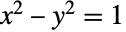 と交わる原点からの放射線と
 軸との間の面積の2倍になるようにすることで定義される.そうすると,Cosh[α]は交点の水平座標を表す.Coshは
 としても定義される.ただし,
 は自然対数Logの底である.
- Coshは,その引数が有理数の(自然)対数であるときは,自動的に厳密値に評価される.引数として厳密な数式が与えられると,Coshは任意の数値精度に評価されることがある.Coshを含む記号式の操作に便利なその他の演算には,TrigToExp,TrigExpand,Simplify,FullSimplifyがある.
- Coshは要素単位でリストおよび行列に縫い込まれる.対照的に,MatrixFunctionを使って,平方行列の双曲線余弦(つまり,通常のベキが行列のベキで置き換えられた双曲線余弦関数のベキ級数)を与えることができる.
- Cosh[x]は,x が
 に近付くにつれて,指数的に増大する.Coshは,Cosによって満足されるような,ピタゴラス(Pythagorean)の恒等式に似た恒等式
 を満足する.双曲線正弦関数の定義は,恒等式
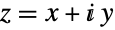
 によって,複素引数
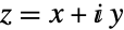 にまで拡張される.双曲線余弦関数は完全である.つまり,複素平面の有限なすべての点において複素微分が可能である.Cosh[z]は,原点付近で級数展開
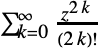 を持つ.
- Coshの逆関数はArcCoshである.他の関連する数学関数にはSinhおよびSechがある.
例題
すべて開く すべて閉じる例 (4)
スコープ (48)
数値評価 (6)
Cosh[1.2]N[Cosh[12 / 10], 50]Cosh[1.20000000000000000000000]Coshは複素数を入力として取ることができる:
Cosh[2.5 + I]Coshを高精度で効率よく評価する:
Cosh[1.2`500]//TimingCosh[1.2`100000];//TimingCosh[{{(π/3)I, -(π/3)I}, {0, -(π/6)I}}]MatrixFunctionを使って行列のCosh関数を計算することもできる:
MatrixFunction[Cosh[#]&, {{(π/3)I, -(π/3)I}, {0, -(π/6)I}}]IntervalオブジェクトとCenteredIntervalオブジェクトを使って最悪の場合に保証される区間を計算する:
Cosh[Interval[{0, Log[3]}]]Cosh[CenteredInterval[-1, 1 / 100]]Cosh[CenteredInterval[2 + 3I, (1 + I) / 100]]Aroundを使って平均的な場合の統計区間を計算することもできる:
Cosh[Around[(2/Sqrt[3]), 0.1]]特定の値 (4)
固定された純粋な虚点におけるCoshの値:
Table[Cosh[I (π/6) n], {n, -3, 3}]Cosh[Infinity]Cosh[ComplexInfinity]Coshの最小値:
Cosh[0]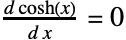
sol = Solve[D[Cosh[x], x] == 0, x, Reals]xmin = x /. First[sol]Plot[Cosh[x], {x, -1, 1}, Epilog -> Style[Point[{xmin, Cosh[xmin]}], PointSize[Large], Red]]Cosh[I Pi / 5]より複雑な場合は明示的にFunctionExpandを使う必要がある:
Cosh[I Pi / 24]FunctionExpand[%]可視化 (3)
Cosh関数をプロットする:
Plot[Cosh[x], {x, -3, 3}]
ComplexContourPlot[Re[Cosh[z]], {z, -3 - 4 I, 3 + 4 I}, IconizedObject[«PlotOptions»]]
ComplexContourPlot[Im[Cosh[z]], {z, -3 - 4 I, 3 + 4 I}, IconizedObject[«PlotOptions»]]
Table[PolarPlot[Cosh[k ϕ], {ϕ, -π, π}, Sequence[Frame -> True, PlotLabel -> "k=" <> ToString[k], PlotRange -> {{-10, 10}, {-40, 40}}, AspectRatio -> 0.8]], {k, 1, 4}]関数の特性 (12)
Coshはすべての実数値と虚数値について定義される:
FunctionDomain[Cosh[x], x]FunctionDomain[Cosh[z], z, Complexes]Coshは1以上のすべての実数値に達する:
FunctionRange[Cosh[x], x, y]FunctionRange[Cosh[z], z, y, Complexes]Coshは偶関数である:
Cosh[-x]Coshは鏡特性 を有する:
FullSimplify[Cosh[Conjugate[z]] == Conjugate[Cosh[z]]]Coshは x の解析関数である:
FunctionAnalytic[Cosh[x], x]Coshは非減少でも非増加でもない:
FunctionMonotonicity[Cosh[x], x]Coshは単射ではない:
FunctionInjective[Cosh[x], x]Plot[{Cosh[x], 5}, {x, -4, 4}]Coshは全射ではない:
FunctionSurjective[Cosh[x], x]Plot[{Cosh[x], -1}, {x, -2, 2}]Coshは非負である:
FunctionSign[Cosh[x], x]FunctionSingularities[Cosh[x], x]FunctionDiscontinuities[Cosh[x], x]Coshは凸である:
FunctionConvexity[Cosh[x], x]TraditionalFormによる表示:
Cosh[x]//TraditionalForm微分 (3)

 次導関数の式:
積分 (4)
Coshの不定積分:
Integrate[Cosh[x], x]Coshを含む三角関数の積の不定積分:
Integrate[Sinh[x]Cosh[x], x]原点を中心とした区間上のCoshの定積分:
Integrate[Cosh[x], {x, -1, 1}]2 Integrate[Cosh[x], {x, 0, 1}]Table[Integrate[Cosh[x ^ n], x], {n, 3}]Integrate[Cosh[x] ^ a, x]級数展開 (4)
Seriesを使ってテイラー(Taylor)展開を求める:
Series[Cosh[x], {x, 0, 7}] の周りのCoshの最初の3つの近似をプロットする:
terms = Normal@Table[Series[Cosh[x], {x, 0, m}], {m, 2, 6, 2}];
Plot[{Cosh[x], terms}, {x, -5, 5}]Coshの級数展開における一般項:
SeriesCoefficient[Cosh[x], {x, 0, n}]Coshのフーリエ(Fourier)級数の最初の数項:
FourierSeries[Cosh[x], x, 2]Coshはベキ級数に適用できる:
Cosh[x + (x^2/2) + (x^3/9) + O[x]^4]積分変換 (2)
LaplaceTransformを使ってラプラス変換を計算する:
LaplaceTransform[Cosh[t], t, s]HankelTransform[Cosh[r], r, s]%//FullSimplify関数の恒等式と簡約 (6)
倍角のCosh:
Expand[Cosh[2x], Trig -> True]総和のCosh:
TrigExpand[Cosh[x + y]]TrigExpand[Cosh[4x]]TrigReduce[%]TrigFactor[Cosh[x] + Cosh[y]]

ComplexExpand[Cosh[x + I y]]TrigToExp[Cosh[z]]関数表現 (4)
Cosを介した表現:
Simplify[Cos[I y]]FullSimplify[I Sqrt[( x/2 Pi)]BesselK[(1/2), -x] + Sqrt[( x/2 Pi)]BesselK[(1/2), x], x > 0]Simplify[Sqrt[( π x/2)]BesselI[-(1/2), x]]MeijerGによる表現:
MeijerGReduce[Cosh[x], x]Activate[%]//FullSimplifyCoshはDifferentialRootとして表すことができる:
DifferentialRootReduce[Cosh[x], x]アプリケーション (10)
ParametricPlot[{Sinh[t], Cosh[t]}, {t, -1, 1}]MatrixPower[{{1, θ / n}, {θ / n, 1}}, n]Limit[%, n -> Infinity]//FullSimplifyΛ = {{Cosh[η], 0, 0, Sinh[η]}, {0, 1, 0, 0}, {0, 0, 1, 0}, {Sinh[η], 0, 0, Cosh[η]}}この行列はミンコフスキー(Minkowski)計量について直交する:
g = DiagonalMatrix[{1, 1, 1, -1}];
FullSimplify[Transpose[Λ].g.Λ]Simplify[With[{η = ArcTanh[v / c]}, {{Cosh[η], -Sinh[η]}, {-Sinh[η], Cosh[η]}}.{c t, x}], 0 < v < c]Series[%, {c, Infinity, 0}]//Normalu[x_, t_] = 4 ArcTan[(c/Sqrt[1 - c^2] ) (Sin[Sqrt[1 - c^2]t]/Cosh[c x])] ;D[u[x, t], t, t] - D[u[x, t], x, x] + Sin[u[x, t]]//FullSimplifySeries[Cosh[t a] == Cosh[t b] Cosh[t c], {t, 0, 2}]Simplify[Normal[%], t > 0]DSolve[-Cos[x]^2 y[x] + Tan[x] Derivative[1][y][x] + Derivative[2][y][x] == 0, y[x], x]DSolve[{y'[t] - 2 y[t] == 0}, y[t], t]ExpToTrig[%]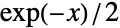


AsymptoticLess[Cosh[x] - Exp[-x] / 2, 1, x -> -∞]ContourPlot[x ^ 2 - y ^ 2 == 1, {x, -5, 5}, {y, -5, 5}, Epilog -> Style[Point[{Cosh[π / 2], Sinh[π / 2]}], PointSize[Large], Red], Axes -> True, Frame -> False, AxesLabel -> {x, y}]特性と関係 (12)
Coshの基本的なパリティと周期性の特性は自動的に適用される:
Cosh[x + 2Pi I]{Cosh[-x], Cosh[I x]}Cosh[x] ^ 2 - Sinh[x] ^ 2Simplifyを使う:
Simplify[%]{Cosh[ArcCosh[z]], Cosh[2ArcCosh[z]], Cosh[3ArcCosh[z]]}FunctionExpand[%]Reduce[Cosh[z]^2 + Cosh[z + 1] == 1, z]FindRoot[Cosh[z]^3 - 3 Cosh[z + 1] + z == 2, {z, 0}]Reduce[Cosh[a x + b] == 0, x]Table[Integrate[Cosh[x ^ n], x], {n, 3}]∫Cosh[z]^aⅆzFourierSinTransform[1 / (Cosh[t] + 1), t, s]Coshは多くの数学関数の特殊形に現れる:
{BesselI[-(1/2), z], JacobiCD[I z, 0], Hypergeometric0F1[(1/2), z], MeijerG[{{}, {(1/2)}}, {{0}, {(1/2), (1/2)}}, z]}Coshは数値関数である:
Attributes[Cosh]NumericQ[Cosh[2 + E]]Coshの母関数:
GeneratingFunction[Cosh[n], n, x]Coshの指数母関数:
ExponentialGeneratingFunction[Cosh[n], n, x]考えられる問題 (5)
Cosh[10. ^ 40 I]N[Cosh[10 ^ 40 I], 20]$MaxExtraPrecisionの設定値を大きくする必要があるかもしれない:
N[Cosh[10 ^ 100 I], 20]
Block[{$MaxExtraPrecision = 200}, N[Cosh[10 ^ 100 I], 20]]Cosh[10. ^ 3]MachineNumberQ[%]無限大ではベキ級数は存在せず,Coshは真性特異点を持つ:
Series[Cosh[x], {x, Infinity, 2}]TraditionalFormでは,引数の周りに丸カッコが必要である:
cosh xcosh(x)
 MathWorld

 The Wolfram Functions Site

 NKS|Online
テキスト
Wolfram Research (1988), Cosh, Wolfram言語関数, https://reference.wolfram.com/language/ref/Cosh.html (2021年に更新).
CMS
Wolfram Language. 1988. "Cosh." Wolfram Language & System Documentation Center. Wolfram Research. Last Modified 2021. https://reference.wolfram.com/language/ref/Cosh.html.
APA
Wolfram Language. (1988). Cosh. Wolfram Language & System Documentation Center. Retrieved from https://reference.wolfram.com/language/ref/Cosh.html