CreateSystemModel[sys]
根据系统模型 sys 创建一个 Modelica SystemModel.
CreateSystemModel[eqns,t]
创建自变量为 t 的系统方程 eqns 的模型.
CreateSystemModel[…,tspec]
创建变量和参数类型指定为 tspec 的模型.
CreateSystemModel[…,spec]
创建一个模型,其中参数值、初始值和模型关系由 spec 给出.
CreateSystemModel
CreateSystemModel[sys]
根据系统模型 sys 创建一个 Modelica SystemModel.
CreateSystemModel[eqns,t]
创建自变量为 t 的系统方程 eqns 的模型.
CreateSystemModel[…,tspec]
创建变量和参数类型指定为 tspec 的模型.
CreateSystemModel[…,spec]
创建一个模型,其中参数值、初始值和模型关系由 spec 给出.
更多信息和选项
- CreateSystemModel 返回 SystemModel[…].
- CreateSystemModel["NewModel",…] 将创建的模型命名为 "NewModel".
- CreateSystemModel["PackageA.NewModel"] 把 "NewModel" 插入到 "PackageA" 中.
- 可能的动态系统模型 sys 包括 StateSpaceModel、TransferFunctionModel、AffineStateSpaceModel、NonlinearStateSpaceModel 和 DiscreteInputOutputModel. »
- 可能的静态系统模型 sys 包括 FittedModel、NetChain 和 NetGraph.
- 可能的方程 eqns 包括常微分方程 (ODE)、微分代数方程 (DAE)、初始值方程和 WhenEvent 给出的事件指定. »
- eqns 和 sys 中的参数被认为是不明确依赖于 t 的变量.
- 变量和参数的类型指定 tspecs 为 {tspec1,…},其中每个 tspeci 的格式为:
-
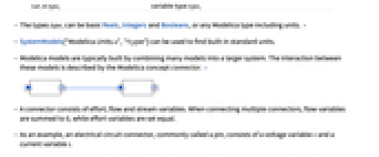
pari∈typei 参数类型 typei vari∈typei 变量类型 typei - 类型 typei 可以为基本的 Reals、Integers 和 Booleans,或任意带有单位的 Modelica 类型. »
- SystemModels["Modelica.Units.*","type"] 可用于查找内置标准单位.
- 一般情况下,通过将许多模型组合成更大的系统来构建 Modelica 模型. 这些模型之间的交互连接则由 Modelica 中的概念 connector 描述. »
- 接口由力和流变量组成. 当把多个接口连在一起时,流变量的和为 0,而力变量被设为相等.
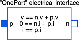
- 举例来说,电路接口常被称为引脚 (pin),由电压变量 v 和电流变量 i 组成.
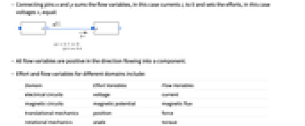
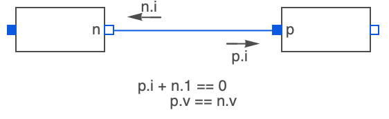
- 将引脚 n 和 p 连接在一起,流变量(这里为电流 i)相加为 0,力(这里为电压 v)则被设为相等:
- 所有流入元件的流变量为正.
- 不同域的力和流变量包括:
-
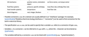
域 力变量 流变量 电路 电压 电流 磁路 磁位 磁通量 平移力学 位置 力 转动力学 角度 转矩 三维力学 位置向量,定向对象 切割力向量,切割扭矩向量 流体流动系统 压力,比焓 质量流率,焓流率 热传导系统 温度 热流率 示意图 实数,整数,布尔值 - - 一个域的可能的接口 conni 通常在 Interfaces 包中被定义. 例如,SystemModels["Modelica.Electrical.Analog.Interfaces.*","connector"] 可用于查找内置电子模型库中的接口.
- 指定 vari∈conni 可用来指定变量 vari 指代类型为 conni 的接口.
- 连接器 c 中的变量 vi 可以用 c▴vi 在 eqns 中引用,其中 ▴ 字符可以输入为 \[UpPointer].
- 可用 SystemModel[conn,"SystemVariables"] 来列出由接口 conn 定义的变量.
- 在 CreateSystemModel[…,spec] 中,spec 是一个 Association,其中的键为:
-
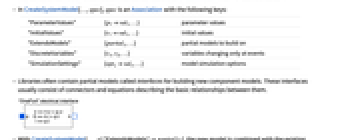
"ParameterValues" {p1val1,…} 参数值 "InitialValues" {v1val1,…} 初始值 "ExtendsModels" {partial1,…} 所基于的部分模型 "DiscreteVariables" {v1,v2,…} 仅在事件发生时变化的变量 "SimulationSettings" {opt1val1,…} 模型仿真选项 - 模型库经常含有被称为 interfaces 的部分模型,可用来构建新的元件模型. 这些界面通常由接口和描述接口间基本关系的方程构成.
- 当设置为 CreateSystemModel[…,"ExtendsModels"partial] 时,会将新模型与 Modelica 中已定义的 partial SystemModel 结合在一起. »
- 通过使用 "ExtendsModels"{"partial1",…} 一个模型可以跨越多个模型.
- 在其上进行构建的部分模通常在 Interfaces 包中被定义. 例如,SystemModels["Modelica.Electrical.Analog.Interfaces.*","model"|"block"] 可用于查找内置电子模型库中的部分模型 (partial models).
- "InitialValues" 对应于 Modelica 模型中的 start 属性.
- 在 "SimulationsSettings"->{opt1val1,…} 中允许的选项包括:
-
"Method" 仿真方法 "StartTime" 仿真开始时间 "StopTime" 仿真停止时间 - 可用的自适应步长 "Method" 值包括:
-
"DASSL" DASSL DAE 求解器 "CVODES" CVODES ODE 求解器 - 自适应步长法的选项包括:
-
"InterpolationPoints" 插值点数 "Tolerance" 自适应步长的公差 - 可用的固定步长 "Method" 值包括:
-
"Euler" 显式 1 阶欧拉方法 "Heun" 2 阶 Heun 方法 "RungeKutta" 显式四阶 Runge-Kutta 法 - 固定步长法的选项包括:
-
"StepSize" 固定步长 - 使用 GeneratedAssetLocationloc 选项,您可以将生成的资源存储在位置 loc 中.

范例
打开所有单元 关闭所有单元基本范例 (3)
基于 StateSpaceModel 创建模型:
CreateSystemModel[StateSpaceModel[{{{0}}, {{1}}, {{1}}, {{0}}}, SamplingPeriod -> None, SystemsModelLabels -> None]]创建一个基于 TransferFunctionModel 的模型,并为其指定一个自定义名称:
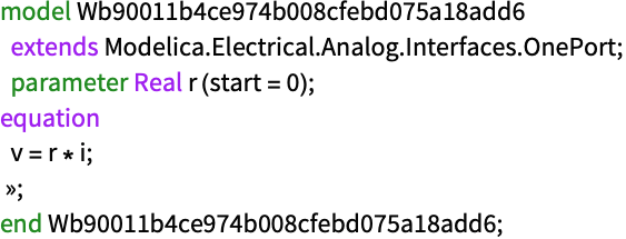
CreateSystemModel["MyTF", TransferFunctionModel[{{{1 + 2*s}}, 1 + s}, s]]model = CreateSystemModel[{v[t] == r i[t]}, t, <|"ExtendsModels" -> "Modelica.Electrical.Analog.Interfaces.OnePort"|>];model["ModelicaDisplay"]范围 (50)
系统模型 (11)
创建一个单入单出模型 TransferFunctionModel:
CreateSystemModel[TransferFunctionModel[{{{1 + 2*s}}, 1 + s}, s]]创建一个单入单出模型 StateSpaceModel:
CreateSystemModel[StateSpaceModel[{{{0}}, {{1}}, {{1}}, {{0}}}, SamplingPeriod -> None, SystemsModelLabels -> None]]CreateSystemModel[TransferFunctionModel[{{{1, 1, 1}, {1, 1, 1}},
{{2 + s, 3 + s, 4 + s},
{3 + s, 4 + s, 5 + s}}}, s]]CreateSystemModel[TransferFunctionModel[{{{p1 + 2*s}}, p2 + s},
s]]CreateSystemModel[StateSpaceModel[{{{a, 0}, {0, b}}, {{1, 0}, {0, 1}}, {{1, 1}}, {{0, 0}}},
SamplingPeriod -> None, SystemsModelLabels -> None]]CreateSystemModel[TransferFunctionModel[{{{p1 + 2*s}}, p2 + s},
s], <|"ParameterValues" -> {p1 -> 1, p2 -> 2}|>]CreateSystemModel[StateSpaceModel[{{{a, 0}, {0, b}}, {{1, 0}, {0, 1}}, {{1, 1}}, {{0, 0}}},
SamplingPeriod -> None, SystemsModelLabels -> None], <|"ParameterValues" -> {a -> 1, b -> 2}|>]CreateSystemModel[StateSpaceModel[{{{a, 0}, {0, b}}, {{1, 0}, {0, 1}}, {{1, 1}}, {{0, 0}}},
SamplingPeriod -> None, SystemsModelLabels -> None], {a∈Reals, b∈"Modelica.Units.SI.Current"}, <|"ParameterValues" -> {a -> 1, b -> 2}|>]CreateSystemModel[TransferFunctionModel[{{{1}}, (-1 + z)*(-0.605 + z)}, z,
SamplingPeriod -> 1]]CreateSystemModel[StateSpaceModel[{{{1, 0, 0}, {0, 2, 0}, {0, 0, 3}}, {{1}, {1}, {1}}, {{1, 1, 1}}, {{0}}},
SamplingPeriod -> 2, SystemsModelLabels -> None]]CreateSystemModel[StateSpaceModel[{{{3, 0}, {0, 4}}, {{5}, {6}}, {{7, 8}}, {{9}}, {{1, 0}, {0, 2}}},
SamplingPeriod -> None, SystemsModelLabels -> None]]CreateSystemModel[AffineStateSpaceModel[{{x2^2, x1 - x2}, {{1}, {1}},
{x1}, {{0}}}, {x1, x2}, Automatic, {Automatic}, Automatic,
SamplingPeriod -> None]]CreateSystemModel[NonlinearStateSpaceModel[{{u1 - x1*x2,
1 + u1*x2}, {x1}}, {x1, x2},
{u1}, {Automatic}, Automatic, SamplingPeriod -> None]]CreateSystemModel[DiscreteInputOutputModel[Association["SampledSeries" -> TemporalData[TimeSeries,
{{{{u1[0]}, {u1[1]}, {u1[2]}}}, {{0, 2, 1}}, 1, {"Discrete", 1}, {"Discrete", 1}, {1},
{MissingDataMethod -> None, ResamplingMethod -> {"Interpolation", Int ... ime", "LastValue", "OutputCount", "OutputVariables", "Path",
"PathComponent", "PathComponents", "PathFunction", "PathLength", "SamplingPeriod", "StateCount",
"TemporalData", "TimePath", "Times", "TimeSeries", "TimeValues", "Type", "Values"}]]微分方程 (12)
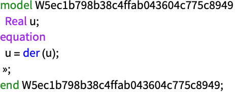
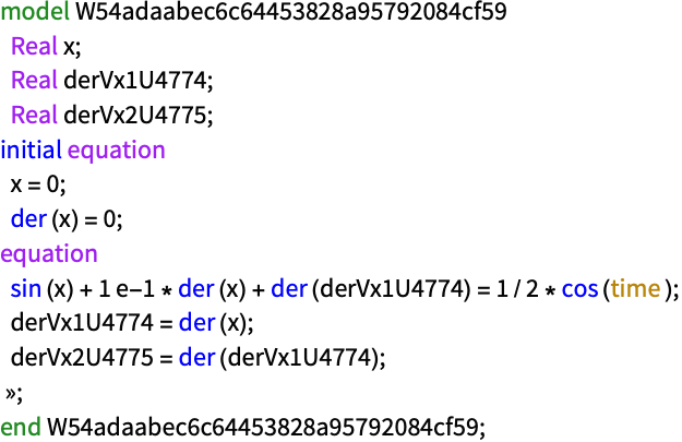
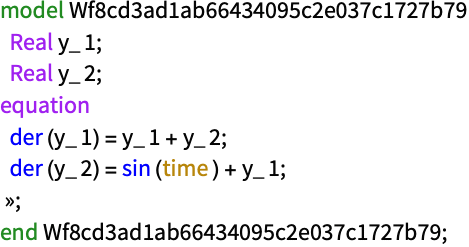
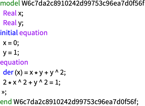
model = CreateSystemModel[{u[t] == u'[t]}, t];model["ModelicaDisplay"]model = CreateSystemModel[{x''[t] + 1 / 10x'[t] + Sin[x[t]] == 1 / 2 Cos[t], x[0] == 0, x'[0] == 0}, t];model["ModelicaDisplay"]model = CreateSystemModel[{Subscript[y, 1]'[t] == Subscript[y, 1][t] + Subscript[y, 2][t], Subscript[y, 2]'[t] == Subscript[y, 1][t] + Sin[t]}, t];model["ModelicaDisplay"]定义一个带有代数约束的方程组,导致高指数 (high-index) 问题:
model = CreateSystemModel[{x'[t] == y[t] ^ 2 + x[t]y[t], 2x[t] ^ 2 + y[t] ^ 2 == 1, x[0] == 0, y[0] == 1}, t];model["ModelicaDisplay"]可用 WhenEvent 指定混合方程:
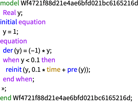
model = CreateSystemModel[{y'[x] == -y[x], WhenEvent[y[x] < 0.1, y[x] -> y[x] + 0.1 * x], y[0] == 1}, x];model["ModelicaDisplay"]sim = SystemModelSimulate[model, 10];SystemModelPlot[sim, {"y"}]eqs = {y''[t] == -9.8, WhenEvent[y[t] - a[t] < 0, y'[t] -> -0.75 y'[t]], WhenEvent[Mod[t, 1] == 0, a[t] -> a[t] - 1], y[0] == 14, y'[0] == 5, a[0] == 13};model = CreateSystemModel[eqs, t, <|"DiscreteVariables" -> {a}|>];sim = SystemModelSimulate[model, 10];SystemModelPlot[sim, {"y", "a"}, Filling -> {2 -> 0}]Wolfram 语言函数会被自动转换为 Modelica 等效模型:
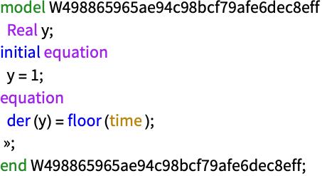
model = CreateSystemModel[{y'[x] == Floor[x], y[0] == 1}, x];model["ModelicaDisplay"]model = CreateSystemModel[{x'[t] == par x[t], x'[0] == 2}, t,
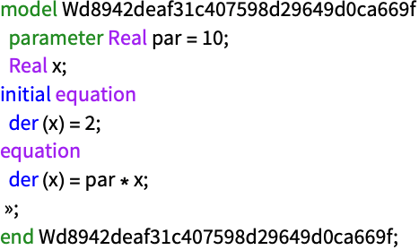
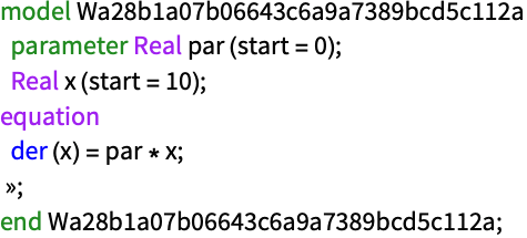
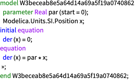
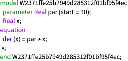
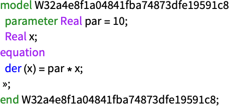
<|"ParameterValues" -> {par -> 10}|>];model["ModelicaDisplay"]model = CreateSystemModel[{x'[t] == par x[t]}, t, <|"InitialValues" -> {x -> 10}|>];model["ModelicaDisplay"]model = CreateSystemModel[{x'[t] == par x[t], x'[0] == 0}, t, {par∈Reals, x∈"Modelica.Units.SI.Position"}];model["ModelicaDisplay"]用 Indexed 表示数组:
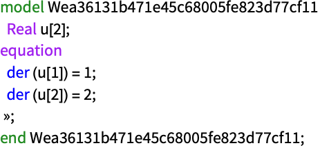
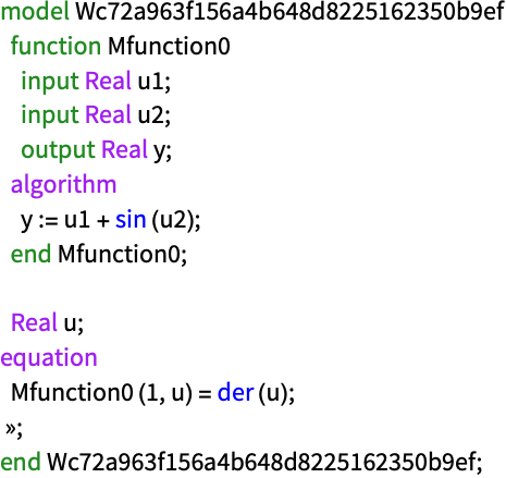
model = CreateSystemModel[{Indexed[u, 1]'[t] == 1, Indexed[u, 2]'[t] == 2}, t];model["ModelicaDisplay"]model = CreateSystemModel[{Unevaluated[Function[#1 + Sin[#2]]][1, u[t]] == u'[t]}, t];model["ModelicaDisplay"]关联和函数 (4)
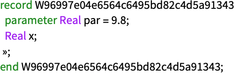
Association 被转换为一条记录:
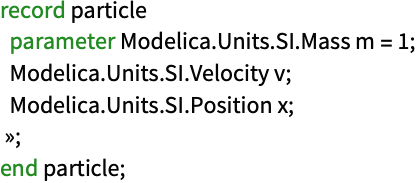
model = CreateSystemModel[<|par -> 9.8, x[t] -> None|>, t];model["ModelicaDisplay"]model = CreateSystemModel["particle", <|m -> 1, x[t] -> None, v[t] -> None|>, t, {"m"∈"Modelica.Units.SI.Mass", "x"∈"Modelica.Units.SI.Position", "v"∈"Modelica.Units.SI.Velocity"}];model["ModelicaDisplay"]创建一个类别,分类规范函数来自 Function:
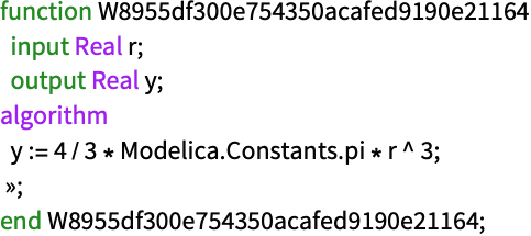
model = CreateSystemModel[Function[r, (4/3)π r^3]];model["ModelicaDisplay"]用 Module 引入保护变量:
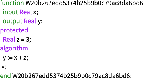
model = CreateSystemModel[Function[x, Module[{z = 3}, x + z]]];model["ModelicaDisplay"]区域和 Graphics3D (2)
model = CreateSystemModel["MyCylinder", Cylinder[]]用 "Modelica.Mechanics.MultiBody" 组件存储如 RegionMeasure、RegionCentroid 和 MomentOfInertia 这样的数据:
model["LocalComponents"]Graphics3D 对象输出,以制作可视化效果:
CreateSystemModel["MyBallCAD", Graphics3D[Ball[]]]DiscretizeGraphics 或 BoundaryDiscretizeGraphics 也许能够从 Graphics3D 生成一个区域:
reg = DiscretizeGraphics[Graphics3D[Ball[]]];CreateSystemModel["ball", reg]拟合模型与神经网络 (2)
使用 FittedModel 创建一个输入-输出块:
data = {{0, 0.5}, {1, 1}, {2, 1.5}, {3, 2}, {4, 2.5}, {5, 3}};nlm = NonlinearModelFit[data, Log[a + b x ^ 2], {a, b}, x]model = CreateSystemModel[nlm]Show[ListPlot[data], SystemModelPlot[model, {"y"}, 5, <|"Inputs" -> {"u" -> Function[t, t]}|>, PlotStyle -> RGBColor[0.880722, 0.611041, 0.142051]]]根据经训练的或初始化的 NetChain 或 NetGraph 创建输入输出模块:
model = CreateSystemModel[NetInitialize[NetChain[{LinearLayer[2, "Input" -> 1]}]]]SystemModelPlot[model, {"y[1]", "y[2]"}, 5, <|"Inputs" -> {"u[1]" -> Sin}|>]模型命名 (3)
model = CreateSystemModel["MySSM", StateSpaceModel[{{{0}}, {{1}}, {{1}}, {{0}}}, SamplingPeriod -> None, SystemsModelLabels -> None]];model["ModelName"]model = CreateSystemModel["MyPackage.MySSM", StateSpaceModel[{{{0}}, {{1}}, {{1}}, {{0}}}, SamplingPeriod -> None, SystemsModelLabels -> None]];model["ModelName"]model = CreateSystemModel[StateSpaceModel[{{{0}}, {{1}}, {{1}}, {{0}}}, SamplingPeriod -> None, SystemsModelLabels -> None]];model["ModelName"]SetSystemModel[model, <|"ModelName" -> "MyModel"|>];model["ModelName"]类型和连接器 (4)
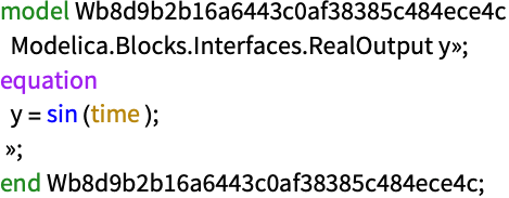
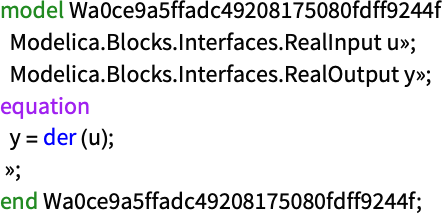
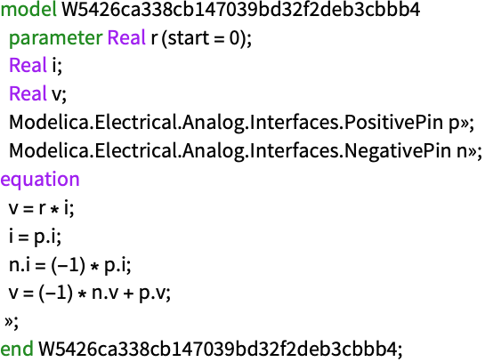
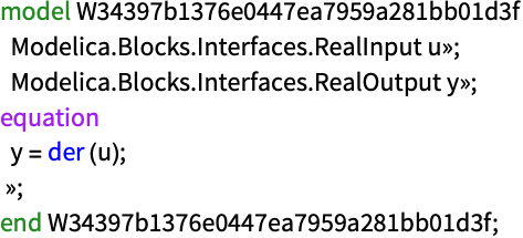
eqs = {y[t] == Sin[t]};conns = {y∈"Modelica.Blocks.Interfaces.RealOutput"};model = CreateSystemModel[eqs, t, conns];model["ModelicaDisplay"]eqs = {y[t] == u'[t]};conns = {u∈"Modelica.Blocks.Interfaces.RealInput", y∈"Modelica.Blocks.Interfaces.RealOutput"};model = CreateSystemModel[eqs, t, conns];model["ModelicaDisplay"]eqs = {v[t] == r i[t], i[t] == QuantityVariable["p.i", "ElectricCurrent"][t], QuantityVariable["n.i", "ElectricCurrent"][t] == -QuantityVariable["p.i", "ElectricCurrent"][t], v[t] == QuantityVariable["p.v", "ElectricPotential"][t] - QuantityVariable["n.v", "ElectricPotential"][t]};model = CreateSystemModel[eqs, t, {p∈"Modelica.Electrical.Analog.Interfaces.PositivePin", n∈"Modelica.Electrical.Analog.Interfaces.NegativePin"}];model["ModelicaDisplay"]conns = {u∈"Interfaces.RealInput", y∈"Interfaces.RealOutput"};model = CreateSystemModel[{y[t] == u'[t]}, t, conns];model["ModelicaDisplay"]初始值和参数值 (6)
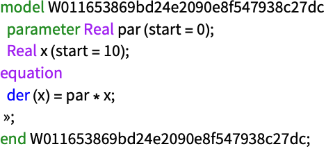
model = CreateSystemModel[{x'[t] == par x[t]}, t, <|"InitialValues" -> {x -> 10}|>];model["ModelicaDisplay"]model = CreateSystemModel[{x'[t] == par x[t]}, t, <|"InitialValues" -> {par -> 10}|>];model["ModelicaDisplay"]如果 start 值和初始化方程同时存在,初始化方程的优先级较高:
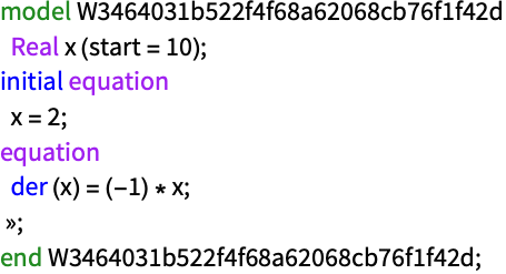
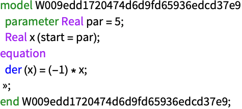
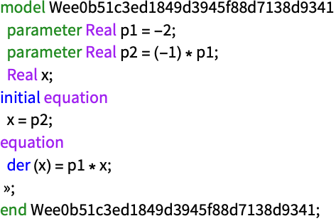
model = CreateSystemModel[{x'[t] == -x[t], x[0] == 2}, t, <|"InitialValues" -> {x -> 10}|>];model["ModelicaDisplay"]SystemModelPlot[model, {"x"}, 5]model = CreateSystemModel[{x'[t] == -x[t]}, t, <|"ParameterValues" -> {par -> 5}, "InitialValues" -> {x -> par}|>];model["ModelicaDisplay"]model = CreateSystemModel[{x'[t] == par x[t]}, t, <|"ParameterValues" -> {par -> 10}|>];model["ModelicaDisplay"]model = CreateSystemModel[{x'[t] == p1 x[t], x[0] == p2}, t, <|"ParameterValues" -> {p1 -> -2, p2 -> -p1}|>];model["ModelicaDisplay"]在部分模型上构建 (3)
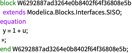
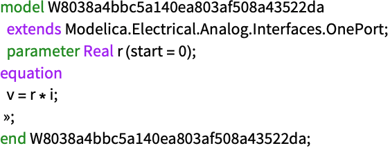
eqs = {y[t] == u[t] + 1};model = CreateSystemModel[eqs, t, <|"ExtendsModels" -> "Blocks.Interfaces.SISO"|>];model["ModelicaDisplay"]model = CreateSystemModel[{v[t] == r i[t]}, t, <|"ExtendsModels" -> "Analog.Interfaces.OnePort"|>];model["ModelicaDisplay"]model = CreateSystemModel[{{"a", ""}, {"b", "b case"}}, <|"ExtendsModels" -> "Enumeration"|>];model["ModelicaDisplay"]仿真设置 (3)
model = CreateSystemModel[{u'[t] == Cos[u[t]]}, t, <|"SimulationSettings" -> {"StartTime" -> 1,
"StopTime" -> 5}|>]SystemModelPlot[model, {"u"}]model = CreateSystemModel[StateSpaceModel[{{{0}}, {{1}}, {{1}}, {{0}}}, SamplingPeriod -> None, SystemsModelLabels -> None], <|"SimulationSettings" -> {"Method" -> "RungeKutta"}|>];model["SimulationSettings"]model = CreateSystemModel[StateSpaceModel[{{{0}}, {{1}}, {{1}}, {{0}}}, SamplingPeriod -> None, SystemsModelLabels -> None], <|"SimulationSettings" -> {"SynchronizeWithRealTime" -> True}|>];model["SimulationSettings"]选项 (2)
GeneratedAssetLocation (2)
默认情况下,从区域创建的模型会将资产文件导出到 $WolframDocumentsDirectory:
model = CreateSystemModel[Cylinder[]]使用 GeneratedAssetLocation 为资源指定一个位置:
model = CreateSystemModel[Cylinder[], GeneratedAssetLocation -> FileNameJoin[{$TemporaryDirectory, "cyl.obj"}]]默认情况下,从神经网络创建的模型将 ONNX 文件导出到 $WolframDocumentsDirectory:
net = NetInitialize[NetChain[{LinearLayer[3, "Input" -> 2]}]];model = CreateSystemModel[net]使用 GeneratedAssetLocation 指定结果的位置:
model = CreateSystemModel[net, GeneratedAssetLocation -> FileNameJoin[{$TemporaryDirectory, "MyNet.onnx"}]]应用 (7)
eqs = {v[t] == h'[t], v'[t] == -9.81, WhenEvent[h[t] ≤ 0, v[t] -> -k v[t]], h[0] == 1};model = CreateSystemModel[eqs, t];sim = SystemModelSimulate[model, 10, <|"ParameterValues" -> {"k" -> 0.95}|>];SystemModelPlot[sim, "h"]创建 Lotka–Volterra 方程的模型,模拟掠食者-猎物关系:
eqs = {pred'[t] == pred[t](δ prey[t] - γ), prey'[t] == prey[t](α - β pred[t])};ieqs = {prey[0] == 10, pred[0] == 10};pars = {α -> 0.1, β -> 0.02, γ -> 0.4, δ -> 0.02};model = CreateSystemModel[Join[eqs, ieqs], t, <|"ParameterValues" -> pars|>];sim = SystemModelSimulate[model, 100];SystemModelPlot[sim, {"pred", "prey"}]sims = SystemModelSimulate[model, 100, <|"ParameterValues" -> {"alpha" -> {0.1, 0.2, 0.3, 0.4}}|>];Partition[Map[SystemModelPlot[#, {"prey", "pred"}, PlotLabel -> α == #["alpha"]]&, sims], 2]//Grid
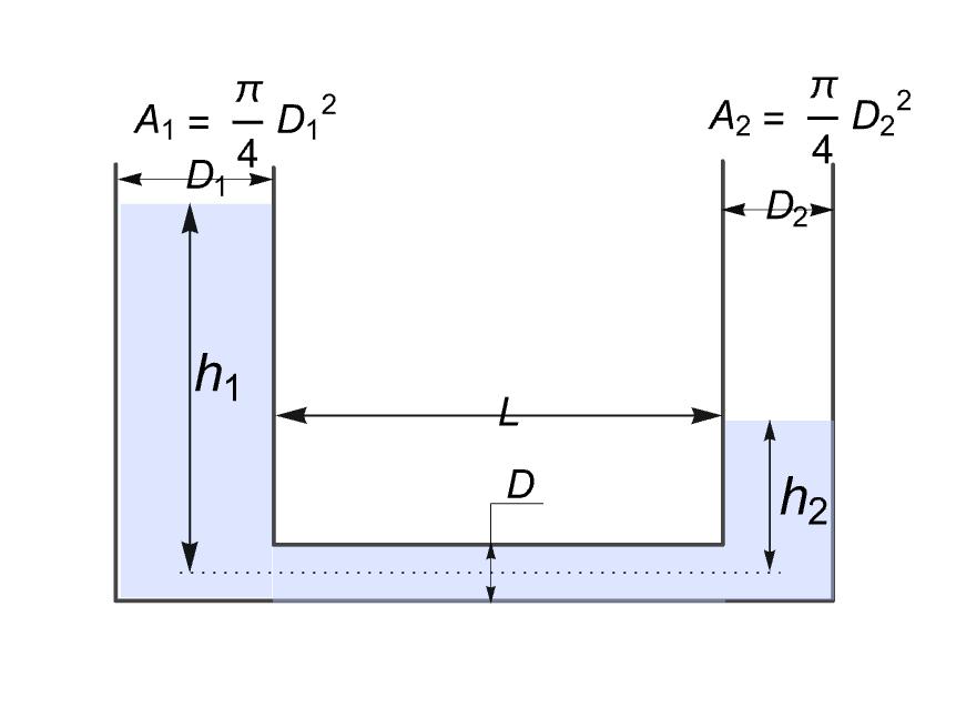
pressureEqns = {p1[t] == ρ g h1[t], p2[t] == ρ g h2[t]};flowRate = (p1[t] - p2[t])(π pipeDia ^ 4) / (128 μ pipeLen);massConservation = {a1 h1'[t] == -flowRate, a2 h2'[t] == flowRate - a2 h2[t] / 10};eqns = Join[pressureEqns, massConservation, {h1[0] == 1, h2[0] == 0}];pars = {pipeLen -> 0.1, pipeDia -> 0.2, ρ -> 0.2, μ -> 2 10 ^ -3, g -> 9.81, a1 -> 1, a2 -> 1};model = CreateSystemModel[eqns, t, <|"ParameterValues" -> pars|>];sim = SystemModelSimulate[model, 80];随着时间的推移,最终两个池子都会被排干,因为第二个池子有泄漏:
SystemModelPlot[sim, {"h1", "h2"}]eqs = {f[t] == If[vrel[t] > 0, d * vrel[t], 0], vrel[t] == s⎵rel'[t]};pvals = {d -> 1};用 Translational Mechanics library 中的部分界面创建阻尼:
partial = "Translational.Interfaces.PartialCompliant";CreateSystemModel["UniDamper", eqs, t, <|"ParameterValues" -> pvals, "ExtendsModels" -> partial|>];model = SystemModel["DocumentationExamples.Modeling.DamperCompare"]sim = SystemModelSimulate[model, 8]SystemModelPlot[sim, {"massUniDir.s", "massBiDir.s"}, PlotRange -> All]a = LeastSquaresFilterKernel[{"Lowpass", 0.1}, 20];h = ListZTransform[a, z];tf = TransferFunctionModel[h, z, SamplingPeriod -> 0.01]//TransferFunctionCancellowpass = CreateSystemModel[tf];signal = CreateSystemModel["Signal", {y[t] == Abs[Sin[t Cos[2t]]]t}, t, <|"ExtendsModels" -> "Modelica.Blocks.Interfaces.SignalSource"|>];model = ConnectSystemModelComponents["FilteredSignal", {"signal"∈signal, "filter"∈lowpass}, {"signal.y""filter.u"}]sim = SystemModelSimulate[model, 10];
SystemModelPlot[sim, {"signal.y", "filter.y"}]将区域与世界的组件一起使用以创建新模型,其中的物体会受到重力影响:
model = CreateSystemModel["MyCylinder", Cylinder[]];model2 = ConnectSystemModelComponents["FallingCylinder", {"cyl"∈"MyCylinder", "world"∈"Modelica.Mechanics.MultiBody.World"
}, {}]sim = SystemModelSimulate[model2, 10];SystemModelPlot[sim, {"cyl.frame_a.r_0[2]"}]book = Parallelepiped[{0, 0, 0}, {{1, 0, 0}, {0, 1 / 2, 0}, {0, 0, 2 / 100}}];model = CreateSystemModel["Book", book]通过更改世界组件中的参数来关闭重力,并为角速度提供一个初始值:
model2 = ConnectSystemModelComponents["RotatingBook", {"book"∈"Book", "world"∈"Modelica.Mechanics.MultiBody.World"}, {}, <|"ParameterValues" -> {"world.gravityType" -> QuantityVariable["Modelica.Mechanics.MultiBody.Types.GravityTypes.NoGravity", IndependentPhysicalQuantity[""]]}, "InitialValues" -> {"book.body.w_a" -> {0.1, 3, 0}}|>]sim = SystemModelSimulate["RotatingBook", 10];ℛ[t_] = {sim[{"book.frame_a.R.T[1,1]", "book.frame_a.R.T[2,1]", "book.frame_a.R.T[3,1]"}, t],
sim[{"book.frame_a.R.T[1,2]", "book.frame_a.R.T[2,2]", "book.frame_a.R.T[3,2]"}, t],
sim[{"book.frame_a.R.T[1,3]", "book.frame_a.R.T[2,3]", "book.frame_a.R.T[3,3]"}, t]};Manipulate[Graphics3D[{EdgeForm[Thick], GeometricTransformation[book, Composition[TranslationTransform[RegionCentroid[book]], LinearFractionalTransform[{ℛ[t]}], TranslationTransform[-RegionCentroid[book]]]]}, PlotRange -> {{-1 / 2, 3 / 2}, {-1 / 2, 3 / 2}, {-1, 1}}, Boxed -> False], {t, 0, 10, 0.1}, SaveDefinitions -> True]属性和关系 (3)
SystemModel 属性可用来从模型中提取信息:
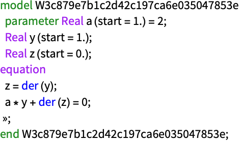
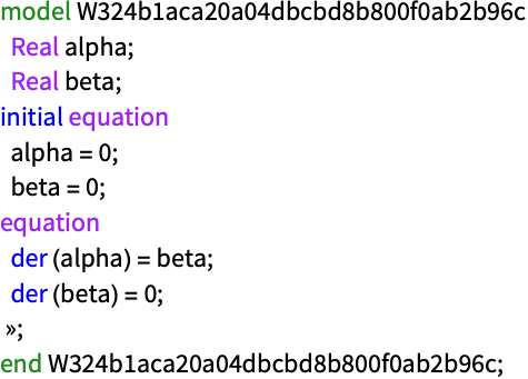
origModel = SystemModel["DocumentationExamples.Basic.DiffEq"];eqs = origModel["SystemEquations", t];ivals = origModel["InitialValues"];newModel = CreateSystemModel[eqs, t, <|"ParameterValues" -> {"a" -> 2}, "InitialValues" -> ivals|>];newModel["ModelicaDisplay"]origSim = SystemModelSimulate[origModel, 5];newSim = SystemModelSimulate[newModel, 5];SystemModelPlot[{origSim, newSim}, {"y", "z"}]model = CreateSystemModel[{α'[t] == β[t], β'[t] == 0, α[0] == 0, β[0] == 0}, t];model["ModelicaDisplay"]Subscript 被转换为 _:
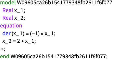
model = CreateSystemModel[{Subscript[x, 1]'[t] == -Subscript[x, 1][t], Subscript[x, 2][t] == 2Subscript[x, 1][t]}, t];model["ModelicaDisplay"]可能存在的问题 (2)
model = CreateSystemModel["NoSave", {x'[t] == par x[t]}, t];Quit[]SystemModel["NoSave", "Summary"]CreateSystemModel 支持 Wolfram 语音函数的子集:
CreateSystemModel[{Subscript[x, 1]'[t] == Gamma[Subscript[x, 1][t]]}, t]文本
Wolfram Research (2018),CreateSystemModel,Wolfram 语言函数,https://reference.wolfram.com/language/ref/CreateSystemModel.html (更新于 2022 年).
CMS
Wolfram 语言. 2018. "CreateSystemModel." Wolfram 语言与系统参考资料中心. Wolfram Research. 最新版本 2022. https://reference.wolfram.com/language/ref/CreateSystemModel.html.
APA
Wolfram 语言. (2018). CreateSystemModel. Wolfram 语言与系统参考资料中心. 追溯自 https://reference.wolfram.com/language/ref/CreateSystemModel.html 年
BibTeX
@misc{reference.wolfram_2026_createsystemmodel, author="Wolfram Research", title="{CreateSystemModel}", year="2022", howpublished="\url{https://reference.wolfram.com/language/ref/CreateSystemModel.html}", note=[Accessed: 07-September-2026]}
BibLaTeX
@online{reference.wolfram_2026_createsystemmodel, organization={Wolfram Research}, title={CreateSystemModel}, year={2022}, url={https://reference.wolfram.com/language/ref/CreateSystemModel.html}, note=[Accessed: 07-September-2026]}