DEigensystem[ℒ[u[x,y,…]],u,{x,y,…}∈Ω,n]
给出线性微分算子 ℒ 在区域 Ω 上 n 个幅值最小的特征值和特征函数.
DEigensystem[eqns,u,t,{x,y,…}∈Ω,n]
给出含时微分方程 eqns 的解 u 的特征值和特征函数.
DEigensystem
DEigensystem[ℒ[u[x,y,…]],u,{x,y,…}∈Ω,n]
给出线性微分算子 ℒ 在区域 Ω 上 n 个幅值最小的特征值和特征函数.
DEigensystem[eqns,u,t,{x,y,…}∈Ω,n]
给出含时微分方程 eqns 的解 u 的特征值和特征函数.
更多信息和选项
- DEigensystem 可以根据边界条件,计算常微分算子和偏微分算子的特征值和特征函数.
- DEigensystem 给出特征值 λi 和特征函数 ui 的列表 {{λ1,…,λn},{u1,…,un}}.
- 微分算子 ℒ 的特征值和特征函数对 {λi,ui} 满足 ℒ[ui[x,y,…]]==λi ui[x,y,…].
- 可以包含齐次 DirichletCondition 或 NeumannValue 边界条件. 非齐次边界条件将被相应的齐次边界条件代替.
- 如果没有指定边界 ∂Ω 处的边界条件,则相当于指定诺伊曼 0 边界条件.
- 方程 eqns 的规范与在 DSolve 中的一样.
- 对于不能符号式计算特征系统,N[DEigensystem[…]] 会调用 NDEigensystem.
- 可以给出下列选项:
-
Assumptions $Assumptions 对参数的假设 Method Automatic 使用的方法 - 特征函数不会自动归一化. 设置 Method->"Normalize" 可被用于给出归一化的特征函数.
范例
打开所有单元 关闭所有单元基本范例 (2)
求拉普拉斯算子在 [0,π] 上 4 个最小的特征值和特征函数:
DEigensystem[{-Laplacian[u[x], {x}], DirichletCondition[u[x] == 0, True]}, u[x], {x, 0, π}, 4]Plot[Evaluate[%[[2]]], {x, 0, π}]{vals, funs} = DEigensystem[{-Laplacian[u[x, y], {x, y}], DirichletCondition[u[x, y] == 0, True]}, u[x, y], {x, y}∈Disk[], 6];vals//NTable[Plot3D[funs[[i]]//N//Evaluate, {x, y}∈Disk[], PlotRange -> All, PlotLabel -> vals[[i]], PlotTheme -> "Minimal"], {i, Length[vals]}]范围 (20)
1D (9)
ℒ = -Laplacian[u[x], {x}];ℬ = DirichletCondition[u[x] == 0, True];{vals, funs} = DEigensystem[{ℒ, ℬ}, u[x], {x, 0, π}, 5];valsPlot[Evaluate[funs], {x, 0, π}]ℒ = -Laplacian[u[x], {x}];ℬ = NeumannValue[0, True];{vals, funs} = DEigensystem[ℒ + ℬ, u[x], {x, 0, π}, 5];vals{vals, funs} = DEigensystem[ℒ, u[x], {x, 0, π}, 5];valsℒ = -Laplacian[u[x], {x}];ℬ1 = DirichletCondition[u[x] == 0, x == 0];ℬ2 = NeumannValue[0, x == π];{vals, funs} = DEigensystem[{ℒ + ℬ2, ℬ1}, u[x], {x, 0, π}, 5];valsPlot[Evaluate[funs], {x, 0, π}]ℒ = -Laplacian[u[x], {x}];ℬ1 = DirichletCondition[u[x] == 0, x == π];ℬ2 = NeumannValue[-u[x] / 3, x == 0];{vals, funs} = DEigensystem[{ℒ + ℬ2, ℬ1}, u[x], {x, 0, π}, 5];vals[[1]]//TraditionalFormPlot[Evaluate[funs], {x, 0, π}]ℒ = -Laplacian[u[x], {x}] + x u[x];ℬ = DirichletCondition[u[x] == 0, True];{vals, funs} = DEigensystem[{ℒ, ℬ}, u[x], {x, 0, 1}, 5];vals[[1]]//TraditionalFormPlot[Evaluate[funs], {x, 0, 1}]ℒ = -Laplacian[u[x], {x}] + x u[x];ℬ = NeumannValue[0, True];{vals, funs} = DEigensystem[{ℒ + ℬ}, u[x], {x, 0, 1}, 5];vals[[1]]//TraditionalFormPlot[Evaluate[funs], {x, 0, 1}]{vals, funs} = DEigensystem[{-Laplacian[u[x], {x}], DirichletCondition[u[x] == 0, True]}, u[x], {x, a, b}, 3];valsfunsqho = -(ℏ^2/2m)Laplacian[u[x], {x}] + (m ω^2/2)x ^ 2 u[x];DEigensystem[qho, u[x], {x, -∞, ∞}, 4, Assumptions -> ℏ > 0 && m > 0 && ω > 0]{ℒ, ℬ} = {D[u[t, x], t] == Laplacian[u[t, x], {x}], DirichletCondition[u[t, x] == 0, True]};{vals, funs} = DEigensystem[{ℒ, ℬ}, u[t, x], t, {x, 0, π}, 4]Table[Plot3D[funs[[i]]//Evaluate, {x, -3, 3}, {t, 0, 1 / 3}, PlotRange -> All, Ticks -> False, Mesh -> False], {i, 4}]二维 (6)
{ℒ, ℬ} = {-Laplacian[u[x, y], {x, y}], DirichletCondition[u[x, y] == 0, True]};{vals, funs} = DEigensystem[{ℒ, ℬ}, u[x, y], {x, 0, π}, {y, 0, π}, 9];valsPlot3D[#, {x, 0, π}, {y, 0, π}]& /@ funsℒ = -Laplacian[u[x, y], {x, y}] + NeumannValue[0, True];{vals, funs} = DEigensystem[ℒ, u[x, y], {x, 0, π}, {y, 0, π}, 4];valsfunsContourPlot[#, {x, 0, π}, {y, 0, π}]& /@ funsℒ = -Laplacian[u[x, y], {x, y}];ℬ = DirichletCondition[u[x, y] == 0, True];{vals, funs} = DEigensystem[{ℒ, ℬ}, u[x, y], {x, y}∈Disk[], 4];vals//TraditionalFormContourPlot[#, {x, y}∈Disk[], Contours -> 10]& /@ N[funs]ℒ = -Laplacian[u[x, y], {x, y}] + (x ^ 2 + y ^ 2)u[x, y];ℬ = DirichletCondition[u[x, y] == 0, True];{vals, funs} = DEigensystem[{ℒ, ℬ}, u[x, y], {x, y}∈FullRegion[2], 6];valsTable[ContourPlot[funs[[i]], {x, y}∈Rectangle[{-3, -3}, {3, 3}]], {i, 6}]ℒ = -Laplacian[u[x, y], {x, y}];ℬ = DirichletCondition[u[x, y] == 0, True];{vals, funs} = DEigensystem[{ℒ, ℬ}, u[x, y], {x, y}∈Triangle[], 6];valsTable[Plot3D[funs[[i]], {x, y}∈Triangle[], Boxed -> False, Axes -> False], {i, 6}]ℒ = -Laplacian[u[x, y], {x, y}];ℬ = DirichletCondition[u[x, y] == 0, True];{vals, funs} = DEigensystem[{ℒ, ℬ}, u[x, y], {x, y}∈Disk[{0, 0}, 1, {0, Pi / 5}], 4];vals//TraditionalFormContourPlot[#, {x, y}∈Disk[{0, 0}, 1, {0, Pi / 5}]]& /@ N[funs]//Quiet三维 (5)
ℒ = -Laplacian[u[x, y, z], {x, y, z}];ℬ = DirichletCondition[u[x, y, z] == 0, True];{vals, funs} = DEigensystem[{ℒ, ℬ}, u[x, y, z], {x, y, z}∈Cuboid[{2, 1, 1}, {4, 2, 3}], 7];valsContourPlot3D[Evaluate[funs[[7]]], {x, 2, 4}, {y, 1, 2}, {z, 1, 3}, Boxed -> False, Axes -> False]ℒ = -Laplacian[u[x, y, z], {x, y, z}];ℬ = DirichletCondition[u[x, y, z] == 0, True];{vals, funs} = DEigensystem[{ℒ, ℬ}, u[x, y, z], {x, y, z}∈Cylinder[{{0, 0, 0}, {0, 0, 5}}, 2], 7];vals[[1 ;; 5]]//TraditionalFormDensityPlot3D[funs[[7]]//N//Evaluate, {x, y, z}∈Cylinder[{{0, 0, 0}, {0, 0, 5}}, 2], Boxed -> False, Axes -> False]ℒ = -Laplacian[u[x, y, z], {x, y, z}];ℬ = DirichletCondition[u[x, y, z] == 0, True];{vals, funs} = DEigensystem[{ℒ, ℬ}, u[x, y, z], {x, y, z}∈Ball[{0, 0, 0}, 2], 7];DensityPlot3D[funs[[7]]//N//Evaluate, {x, y, z}∈Ball[{0, 0, 0}, 2], Boxed -> False, Axes -> False, ColorFunction -> Hue]ℒ = -Laplacian[u[x, y, z], {x, y, z}];ℬ = DirichletCondition[u[x, y, z] == 0, True];{vals, funs} = DEigensystem[{ℒ, ℬ}, u[x, y, z], {x, y, z}∈Prism[{{0, 0, 0}, {1, 0, 0}, {0, 1, 0}, {0, 0, 2}, {1, 0, 2}, {0, 1, 2}}], 7];valsDensityPlot3D[funs[[7]]//N//Evaluate, {x, y, z}∈Prism[{{0, 0, 0}, {1, 0, 0}, {0, 1, 0}, {0, 0, 2}, {1, 0, 2}, {0, 1, 2}}], Boxed -> False, ColorFunction -> Hue, PlotPoints -> 50, Axes -> False]ℒ = -Laplacian[u[x, y, z], {x, y, z}] + 2(x^2 + y^2 + z^2)u[x, y, z];ℬ = DirichletCondition[u[x, y, z] == 0, True];{vals, funs} = DEigensystem[{ℒ, ℬ}, u[x, y, z], {x, y, z}∈FullRegion[3], 8];valsTable[DensityPlot3D[funs[[i]]//N//Evaluate, {x, y, z}∈Ball[{0, 0, 0}, 3], Boxed -> False, ColorFunction -> Hue, PlotPoints -> 50, Axes -> False], {i, 8}]选项 (2)
Assumptions (1)
用 Assumptions 化简结果:
DEigensystem[-Laplacian[u[x, y, z], {x, y, z}] + 2ω^2(x^2 + y^2 + z^2)u[x, y, z], u[x, y, z], {x, y, z}∈FullRegion[3], 4, Assumptions -> ω > 0]DEigensystem[-Laplacian[u[x, y, z], {x, y, z}] + 2ω^2(x^2 + y^2 + z^2)u[x, y, z], u[x, y, z], {x, y, z}∈FullRegion[3], 4]应用 (3)
给定在区间
上的狄利克雷条件,计算函数
关于由一维拉普拉斯算子提供的基的特征函数展开式的前三项:
basis = DEigensystem[{-Laplacian[u[x], {x}] + u[x], DirichletCondition[u[x] == 0, True]}, u[x], {x, 0, π}, 3, Method -> "Normalize"][[2]]f[x_] := x ^ 2(π - x) ^ 3coeffs = Table[Integrate[f[x] basis[[i]], {x, 0, Pi}], {i, 3}]eigexp[x_] = Sum[coeffs[[i]]basis[[i]], {i, 3}]Plot[{f[x], eigexp[x]}//Evaluate, {x, 0, Pi}]给定狄利克雷条件,通过使用热方程特征函数的线性组合建立热方程的解:
eqns = {D[u[t, x], t] == Laplacian[u[t, x], {x}], DirichletCondition[u[t, x] == 0, True]};eigfuns = DEigensystem[eqns, u[t, x], t, {x, 0, Pi}, 5][[2]]sol[t_, x_] = Sum[RandomInteger[{1, 10}] eigfuns[[i]], {i, 5}]eqns[[1]] /. {u -> sol}{sol[t, 0], sol[t, π]}Plot3D[sol[t, x], {x, 0, Pi}, {t, 0, 0.7}, PlotRange -> All]实验中,一个 CO 分子根据其平衡长度震荡,震荡的有效弹性系数为
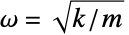
. 震荡由量子谐振方程决定. 在下式中,
是分子的缩减质量,
是自然频率,
是距离平衡位置的位移,而
是缩减的普朗克常数:
qho = -(ℏ^2/2m)Laplacian[u[x], {x}] + (m ω^2/2)x ^ 2 u[x];{ℰs, efuns} = DEigensystem[qho, u[x], {x, -∞, ∞}, 4, Assumptions -> ℏ > 0 && m > 0 && ω > 0, Method -> "Normalize"]ψ[x_, t_] = Total[MapThread[(1/2)Exp[I t #1 / ℏ]#2&, {ℰs, efuns}]]使用原子质量单位的基本单位、飞秒和皮米计算
、
和
,这样能给出接近正常的数量级的值:
m = QuantityMagnitude[(Entity["Element", "Carbon"][EntityProperty["Element", "AtomicMass"]]Entity["Element", "Oxygen"][EntityProperty["Element", "AtomicMass"]]/Entity["Element", "Carbon"][EntityProperty["Element", "AtomicMass"]] + Entity["Element", "Oxygen"][EntityProperty["Element", "AtomicMass"]]), "AtomicMassUnits"]ω = Sqrt[QuantityMagnitude[Quantity[1.86, "Kilonewtons" / "Meters"], "AtomicMassUnit" / "Femtoseconds" ^ 2] / m]ℏ = QuantityMagnitude[Quantity[1., "ReducedPlanckConstant"], "AtomicMassUnit" * "Picometers" ^ 2 / "Femtoseconds"]特征函数对应的势能
可以可视化,通过改变比例尺来放到带状区域
中:
Show[Plot[Evaluate[ℏ ω efuns + ℰs], {x, -18, 18}], Plot[Evaluate[Append[ℰs, (1/2)m ω^2x^2]], {x, -18, 18}, PlotStyle -> Dashed]]ρ[x_, t_] = FullSimplify[ComplexExpand[Conjugate[ψ[x, t]] ψ[x, t]]]Chop[Integrate[ρ[x, t], {x, -∞, ∞}]]Animate[Plot[ρ[x, t], {x, -25, 25}, PlotRange -> {0, .16}, PlotTheme -> "Detailed", FrameLabel -> Style[x, FontSize -> Larger], PlotLegends -> Placed[{HoldForm[ρ][x, NumberForm[t, {3, 2}]]}, Above]], {t, 0., 5.7}, AnimationRate -> 1, SaveDefinitions -> True, Alignment -> Center]属性和关系 (6)
用 NDEigensystem 求特征值和特征向量的数值:
{ℒ, ℬ} = {-Laplacian[u[x], {x}], DirichletCondition[u[x] == 0, True]};exacteigsys = DEigensystem[{ℒ, ℬ}, u[x], {x, 0, Pi}, 3, Method -> "Normalize"]exacteigsys /. {x -> 0.3}neigsys = NDEigensystem[{ℒ, ℬ}, u[x], {x, 0, Pi}, 3] /. {x -> 0.3}用 DEigenvalues 求微分算子的特征值:
{ℒ, ℬ} = {-Laplacian[u[x], {x}], DirichletCondition[u[x] == 0, True]};{vals, funs} = DEigensystem[{ℒ, ℬ}, u[x], {x, 0, Pi}, 3]valsDEigenvalues[{ℒ, ℬ}, u[x], {x, 0, Pi}, 3]用 DSolve 求解特征值问题:
{ℒ, ℬ} = {-Laplacian[u[x], {x}], DirichletCondition[u[x] == 0, True]};{vals, funs} = DEigensystem[{ℒ, ℬ}, u[x], {x, 0, Pi}, 3]DSolve[{u''[x] + λ u[x] == 0, u[0] == 0, u[π] == 0}, u[x], x]由 DEigensystem 给出的特征函数是正交的:
{ℒ, ℬ} = {-Laplacian[u[x], {x}], DirichletCondition[u[x] == 0, True]};{vals, funs} = DEigensystem[{ℒ, ℬ}, u[x], {x, 0, Pi}, 4]Table[Integrate[funs[[i]] * funs[[j]], {x, 0, Pi}], {i, 1, 4}, {j, 1, i - 1}]//Flatten默认情况下,由 DEigensystem 给出的特征函数系统不是正交归一的:
{ℒ, ℬ} = {-Laplacian[u[x], {x}], DirichletCondition[u[x] == 0, True]};{vals, funs} = DEigensystem[{ℒ, ℬ}, u[x], {x, 0, Pi}, 3]Table[Integrate[funs[[i]] funs[[j]], {x, 0, Pi}], {i, 1, 3}, {j, 1, 3}]//MatrixForm用 Method->"Normalize" 得到正交归一的系统:
{vals, funs} = DEigensystem[{ℒ, ℬ}, u[x], {x, 0, Pi}, 3, Method -> "Normalize"]Table[Integrate[funs[[i]] * funs[[j]], {x, 0, Pi}], {i, 1, 3}, {j, 1, 3}]//MatrixForm如果无法进行符号运算, 应用 N[DEigensystem[...]] 会调用 NDEigensystem:

DEigensystem[{-Laplacian[u[x, y], {x, y}] + E ^ (-x ^ 3 + x) u[x, y], DirichletCondition[u[x, y] == 0, True]}, u[x, y], {x, y}∈Rectangle[], 2]N[%]可能存在的问题 (2)
First[DEigensystem[{-Laplacian[u[x], {x}], DirichletCondition[u[x] == 1, True]}, u[x], {x, 0, 1}, 2]]First[DEigensystem[{-Laplacian[u[x], {x}], DirichletCondition[u[x] == 0, True]}, u[x], {x, 0, 1}, 2]]First[DEigensystem[{-Laplacian[u[x], {x}] + NeumannValue[1, True]}, u[x], {x, 0, 1}, 2]]First[DEigensystem[-Laplacian[u[x], {x}], u[x], {x, 0, 1}, 2]]技术笔记
文本
Wolfram Research (2015),DEigensystem,Wolfram 语言函数,https://reference.wolfram.com/language/ref/DEigensystem.html.
CMS
Wolfram 语言. 2015. "DEigensystem." Wolfram 语言与系统参考资料中心. Wolfram Research. https://reference.wolfram.com/language/ref/DEigensystem.html.
APA
Wolfram 语言. (2015). DEigensystem. Wolfram 语言与系统参考资料中心. 追溯自 https://reference.wolfram.com/language/ref/DEigensystem.html 年
BibTeX
@misc{reference.wolfram_2026_deigensystem, author="Wolfram Research", title="{DEigensystem}", year="2015", howpublished="\url{https://reference.wolfram.com/language/ref/DEigensystem.html}", note=[Accessed: 13-September-2026]}
BibLaTeX
@online{reference.wolfram_2026_deigensystem, organization={Wolfram Research}, title={DEigensystem}, year={2015}, url={https://reference.wolfram.com/language/ref/DEigensystem.html}, note=[Accessed: 13-September-2026]}