


DifferenceQuotient[f,{x,h}]
差分係数
を与える.
DifferenceQuotient[f,{x,n,h}]
複数の差分係数をステップ h で与える.
DifferenceQuotient[f,{x1,n1,h1},{x2,n2,h2},…]
x1,x2,…についての偏差分係数を計算する.
DifferenceQuotient
DifferenceQuotient[f,{x,h}]
差分係数

を与える.
DifferenceQuotient[f,{x,n,h}]
複数の差分係数をステップ h で与える.
DifferenceQuotient[f,{x1,n1,h1},{x2,n2,h2},…]
x1,x2,…についての偏差分係数を計算する.
詳細とオプション
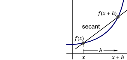
- DifferenceQuotientは,曲線上の近接する2つの点を繋いだ割線の傾きを与える.
- DifferenceQuotient[f,{x,n,h}]は DifferenceDelta[f,{x,n,h}]/
に等しい. - DifferenceQuotient[f,…,Assumptions->assum]は,差分係数の計算過程で仮定 assum を使う.
例題
すべて開く すべて閉じる例 (1)
スコープ (16)
基本的な用法 (4)
DifferenceQuotient[f[x], {x, h}]DifferenceQuotient[f[x], {x, -h}]DifferenceQuotient[f[x - h], {x, 2h}]DifferenceQuotient[f[x], {x, 2, h}]DifferenceQuotient[f[x], {x, 3, h}]DifferenceQuotient[f[x, y], {x, r}, {y, s}]DifferenceQuotientはリストに縫い込まれる:
DifferenceQuotient[{f[x], g[x]}, {x, h}]一変量差分係数 (8)
定数のDifferenceQuotientは0である:
DifferenceQuotient[c, {x, h}]多項式関数のDifferenceQuotientは多項式関数である:
DifferenceQuotient[x ^ 3, {x, h}]Table[DifferenceQuotient[x ^ 4, {x, n, h}], {n, 4}]DifferenceQuotient[(x + 1) / (x + 3), {x, h}]Table[DifferenceQuotient[(x + 1) / (x + 3), {x, n, h}], {n, 2}]DifferenceQuotient[Sin[x], {x, h}]DifferenceQuotient[Cos[2x], {x, h}]Table[DifferenceQuotient[a ^ x, {x, n, h}], {n, 3}]DifferenceQuotient[(x ^ 2 + x + 1)2 ^ x, {x, h}]整数ステップのPolyGammaの差分係数は有理関数である:
Block[{h = 3}, Table[DifferenceQuotient[PolyGamma[n, x], {x, h}], {n, 0, 3}]]HarmonicNumberとZetaについても同様である:
DifferenceQuotient[HarmonicNumber [x, 2], {x, 3}]DifferenceQuotient[Zeta [2, x], {x, 3}]ステップ h のFactorialPowerは a のマッチするステップ h について単純な差分係数を持つ:
DifferenceQuotient[FactorialPower[x, n, h], {x, h}]多変量差分係数 (4)
多変量多項式関数のDifferenceQuotientは多項式関数である:
DifferenceQuotient[x ^ 3 y ^ 2 + 5 x y + 11, {x, h}, {y, k}]DifferenceQuotient[(x + y + 1) / (((x ^ 2 + 3)(y + 5))), {x, h}, {y, k}]DifferenceQuotient[(x + y + 1) / (((x ^ 2 + 3)(y + 5))), {x, 2, h}, {y, 2, k}]変数の部分集合に依存する多変量関数のDifferenceQuotientは0である:
DifferenceQuotient[f[x], {x, h}, {y, k}]DifferenceQuotient[ g[y], {x, h}, {y, k}]DifferenceQuotient[ h[x, y], {x, h}, {y, k}, {z, p}]一変量関数の積についてのDifferenceQuotient:
DifferenceQuotient[f[x] g[y], {x, h}, {y, k}]DifferenceQuotient[f[x], {x, h}]DifferenceQuotient[ g[y], {y, k}]オプション (1)
アプリケーション (10)
第一原理からの導関数 (3)
f[x_] := x ^ 2 + 5x + 7Limit[DifferenceQuotient[f[x], {x, h}], h -> 0]Dを使って導関数を計算する:
f'[x]f[x_] := E ^ (a x)Limit[DifferenceQuotient[f[x], {x, h}], h -> 0]f'[x]f[x_] := Sin[2x + 1]Limit[DifferenceQuotient[f[x], {x, h}], h -> 0]f'[x]f[x_] := x ^ nLimit[DifferenceQuotient[f[x], {x, 2, h}], h -> 0]f''[x]f[x_] := x ^ xLimit[DifferenceQuotient[f[x], {x, 3, h}], h -> 0]f'''[x]//Simplifyf[x_, y_] := Cos[x ^ 2 + E ^ (-y)]Plot3D[f[x, y], {x, -2, 2}, {y, -1, 1}]Limit[DifferenceQuotient[f[x, y], {x, h}], h -> 0]D[f[x, y], x]//SimplifyLimit[DifferenceQuotient[f[x, y], {y, k}], k -> 0]D[f[x, y], y]Limit[Limit[DifferenceQuotient[f[x, y], {x, h}, {y, k}], h -> 0], k -> 0]D[f[x, y], x, y]近似導関数 (3)
DifferenceQuotientを使ってある点で導関数を近似する:
f[x_] := 2 x^3 - 15 x^2 + 33 x - 20Plot[f[x], {x, 0, 5}]f'[2.57]DifferenceQuotientによって与えられる近似:
DifferenceQuotient[f[x], {x, 0.01}] /. {x -> 2.57}f[x_] := Sin[E ^ x]Plot[f[x], {x, 0, π}]f'[2]N[%]hvals = {0.1, 0.01, 0.0001, 0.0001};fd = Table[DifferenceQuotient[f[x], {x, h}], {h, hvals}] /. {x -> 2}bd = Table[DifferenceQuotient[f[x], {x, -h}], {h, hvals}] /. {x -> 2}Table[DifferenceQuotient[f[x - h], {x, 2h}], {h, {0.1, 0.01, 0.0001, 0.0001}}] /. {x -> 2}DifferenceQuotientを使ってある点で偏導関数を近似する:
f[x_, y_] := Sin[x + y]Cos[ 3y]Plot3D[f[x, y], {x, 0, 5}, {y, 0, 5}]{D[f[x, y], {x, 2}], D[f[x, y], x, y], D[f[x, y], {y, 2}]} /. {x -> 2.3, y -> 3.8}{DifferenceQuotient[f[x, y], {x, 2, h}], DifferenceQuotient[f[x, y], {x, h}, {y, k}], DifferenceQuotient[f[x, y], {y, 2, k}]} /. {x -> 2.3, y -> 3.8, h -> 0.001, k -> 0.002}微分方程式 (3)
deqn = {y'[x] == 2x - y[x], y[0] == 5};reqn = {DifferenceQuotient[y[x], {x, 1 / 10}] == 2x - y[x], y[0] == 5}//SimplifyDSolveValueを使って微分方程式を解く:
dsol = DSolveValue[deqn, y[x], x]Plot[dsol, {x, 0, 5}]RSolveValueを使って微分方程式を解く:
rsol = RSolveValue[reqn, y[x], x]//SimplifyTable[dsol, {x, 0., 5}]Table[rsol, {x, 0., 5}]deqn = {y'[x] == 4 - 3y[x], y[0] == 5};reqn = {DifferenceQuotient[y[x], {x, -1 / 10}] == 4 - 3y[x], y[0] == 5}//SimplifyDSolveValueを使って微分方程式を解く:
dsol = DSolveValue[deqn, y[x], x]Plot[dsol, {x, 0, 5}]RSolveValueを使って微分方程式を解く:
rsol = RSolveValue[reqn, y[x], x]//SimplifyTable[dsol, {x, 0., 5}]Table[rsol, {x, 0., 5}]deqn = {y'[x] == x - 3y[x], y[0] == 1};reqn = {DifferenceQuotient[y[x], {x, h}] == x - 3y[x], y[0] == 1}//SimplifyDSolveValueを使って微分方程式を解く:
dsol = DSolveValue[deqn, y[x], x]//SimplifyPlot[dsol, {x, 0, 5}]RSolveValueを使って微分方程式を解く:
rsol[h_] = RSolveValue[reqn, y[x], x]Table[{dsol, rsol[0.1], rsol[-0.1]}, {x, 0., 5}]//TableFormLimit[rsol[h], h -> 0]//FullSimplify補外 (1)
Richardson補外法は母数 h に依存する数列 a[h]の収束率を向上させる一連の加速法である.Richardson補外法を使い,DifferenceQuotientの収束を以下で定義される数列 a[x,h]を使って関数 f[x]の導関数に加速させる:
a[x_, h_] = DifferenceQuotient[f[x], {x, h}]r[x_, h_, k_] = (k ^ 2 a[x, h] - a[x, k h]) / (k ^ 2 - 1)//Simplifyf[x_] := x Sin[E ^ (x)]f'[3.4]DifferenceQuotientで与えられる近似:
a[3.4, 0.001]Table[r[3.4, 0.001, k], {k, {0.5, 0.3, 0.0001}}]特性と関係 (6)
DifferenceQuotientは,曲線上の近接する2点を結んだ割線の傾きを与える:
f[x_] := x ^ 3 + 2x - 5diffquotient = DifferenceQuotient[f[x], {x, h}]% /. {x -> 3, h -> 2}secantslope = (f[5] - f[3]) / 2Show[Plot[f[x], {x, 1, 6}], Graphics[{Red, Line[{{2.5, 2.5}, {5.5, 155.5}}]}]]DifferenceQuotientのLimitは導関数Dである:
DifferenceQuotient[f[x], {x, h}]Limit[%, h -> 0, Analytic -> True]複数の差分係数の反復されたLimitは混合偏微分を与える:
DifferenceQuotient[f[x, y], {x, r}, {y, s}]Limit[Limit[%, r -> 0, Analytic -> True], s -> 0, Analytic -> True]DifferenceQuotientは,
のときにDifferenceDeltaと関連している:
DifferenceQuotient[f[x], {x, h}] == DifferenceDelta[f[x], {x, 1, h}] / h//SimplifyTable[DifferenceQuotient[f[x], {x, n, h}] == DifferenceDelta[f[x], {x, n, h}] / h ^ n//Simplify, {n, 4}]//SimplifyDifferenceQuotientは,
のときにDiscreteShiftと関連している:
DifferenceQuotient[f[x], {x, h}] == (DiscreteShift[f[x], {x, 1, h}] - f[x]) / h//SimplifyDifferenceQuotientは線形演算子である:
DifferenceQuotient[f[x] + g[x], {x, h}] == DifferenceQuotient[f[x], {x, h}] + DifferenceQuotient[g[x], {x, h}]//TogetherDifferenceQuotient[c f[x], {x, h}] == c DifferenceQuotient[f[x], {x, h}]//Togetherインタラクティブな例題 (1)
f[x_] = 10 Exp[-(x^2 - x/4)] Sin[2 x];g[h_, b_][x_] = f[b] + (DifferenceQuotient[f[x], {x, h}] /. (x -> b)) (x - b);割線が関数上での変わり方とすべての点で
の接線となる様子を可視化する:
Manipulate[
Plot[{f[x], g[h, b][x]}, {x, -3, 3}, PlotRange -> 12, Epilog -> {AbsolutePointSize[7], Point[{{b, f[b]}, {b + h, f[b + h]}}]}], {{b, 0}, -2, 2, Appearance -> "Labeled"}, {{h, 1}, -1, 1, Appearance -> "Labeled"}, SaveDefinitions -> True]おもしろい例題 (1)
flist = {1, x, x ^ 2, x ^ 3, 1 / x, Sin[x], Cos[x], Sinh[x], Cosh[x], a ^ (x)};Grid[Transpose[{flist, DifferenceQuotient[flist, {x, h}]}], Dividers -> All, Spacings -> {4, 2}, Background -> StandardBlue, BaseStyle -> {FontFamily -> Times, FontSize -> 13}]//TraditionalForm関連するガイド
-
▪
- 離散微積分 ▪
- 微積分 ▪
- 中学・高校における教育
テキスト
Wolfram Research (2016), DifferenceQuotient, Wolfram言語関数, https://reference.wolfram.com/language/ref/DifferenceQuotient.html.
CMS
Wolfram Language. 2016. "DifferenceQuotient." Wolfram Language & System Documentation Center. Wolfram Research. https://reference.wolfram.com/language/ref/DifferenceQuotient.html.
APA
Wolfram Language. (2016). DifferenceQuotient. Wolfram Language & System Documentation Center. Retrieved from https://reference.wolfram.com/language/ref/DifferenceQuotient.html
BibTeX
@misc{reference.wolfram_2026_differencequotient, author="Wolfram Research", title="{DifferenceQuotient}", year="2016", howpublished="\url{https://reference.wolfram.com/language/ref/DifferenceQuotient.html}", note=[Accessed: 10-September-2026]}
BibLaTeX
@online{reference.wolfram_2026_differencequotient, organization={Wolfram Research}, title={DifferenceQuotient}, year={2016}, url={https://reference.wolfram.com/language/ref/DifferenceQuotient.html}, note=[Accessed: 10-September-2026]}
