ElectricCurrentPDEComponent

ElectricCurrentPDEComponent[vars,pars]

変数 vars，パラメータ pars の電流PDE項を与える．

詳細

ElectricCurrentPDEComponentは，通常，モデル変数 vars，モデルパラメータ pars の電流連続性方程式の生成に使われる．
ElectricCurrentPDEComponentは，偏微分方程式の一部として使われる微分演算子の和を返す．

ElectricCurrentPDEComponentは，定常，周波数，パラメトリックの各解析のためのPDE成分を作成する．
ElectricCurrentPDEComponentは，直流あるいは交流によって作られる電導体内の電場を，磁気および誘導の影響が無視できるという条件のもとにモデル化する．
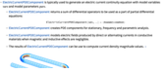
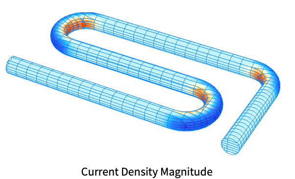
ElectricCurrentPDEComponentの結果を使って電流密度の大きさの値が計算できる． »

ElectricCurrentPDEComponentは，従属変数としての電気スカラーポテンシャル []，独立変数 []で，定常電場あるいは調和電場をモデル化する．
定常変数 vars は vars={V[x₁,…,x_n],{x₁,…,x_n}}である．
時間依存変数 vars は vars={V[t,x₁,…,x_n],t,{x₁,…,x_n}}である．
周波数依存変数 vars は vars={V[x₁,…,x_n],ω,{x₁,…,x_n}}である．
電流連続性方程式はである．ここで，体積電荷密度 [ $TemplateBox[{InterpretationBox[, 1], {"C", , "/", , {"m", ^, 3}}, coulombs per meter cubed, {{(, "Coulombs", )}, /, {(, {"Meters", ^, 3}, )}}}, QuantityTF]$ ]，時間変数 []，電流密度ベクトル [ $TemplateBox[{InterpretationBox[, 1], {"A", , "/", , {"m", ^, 2}}, amperes per meter squared, {{(, "Amperes", )}, /, {(, {"Meters", ^, 2}, )}}}, QuantityTF]$ ]である．
オームの法則としても知られる構成材料モデル方程式は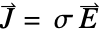である．ここで， []は導電率， []は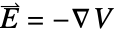の電場である．
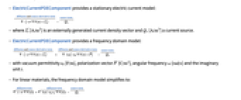
ElectricCurrentPDEComponentは，以下の定常電流モデルを与える．ただし， [ $TemplateBox[{InterpretationBox[, 1], {"A", , "/", , {"m", ^, 2}}, amperes per meter squared, {{(, "Amperes", )}, /, {(, {"Meters", ^, 2}, )}}}, QuantityTF]$ ]は外部的に生成された電流密度ベクトルで， [ $TemplateBox[{InterpretationBox[, 1], {"A", , "/", , {"m", ^, 3}}, amperes per meter cubed, {{(, "Amperes", )}, /, {(, {"Meters", ^, 3}, )}}}, QuantityTF]$ ]は電流弦である．

ElectricCurrentPDEComponentは時間領域モデルを，時間変数 []，真空の誘電率 []，比誘電率 []で与える．

ElectricCurrentPDEComponentは，以下の周波数領域モデルを与える．ただし，真空誘電率 []，は分極ベクトル [ $TemplateBox[{InterpretationBox[, 1], {"C", , "/", , {"m", ^, 2}}, coulombs per meter squared, {{(, "Coulombs", )}, /, {(, {"Meters", ^, 2}, )}}}, QuantityTF]$ ]，角周波数 []，虚数単位である．

線形の材料については，周波数領域モデルは以下のように簡約できる．

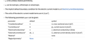
は単位のない比誘電率である．
は，等方性，直交異方性，異方性のいずれかにすることができる．
電流モデルの暗黙的なデフォルトの境界条件は 0 ElectricCurrentDensityValueである．
電流モデル項の単位は[ $TemplateBox[{InterpretationBox[, 1], {"A", , "/", , {"m", ^, 3}}, amperes per meter cubed, {{(, "Amperes", )}, /, {(, {"Meters", ^, 3}, )}}}, QuantityTF]$ ]である．
次は，使用可能なパラメータ pars である．

パラメータ	デフォルト	シンボル
"CrossSectionalArea"	1	，断面積 [ $TemplateBox[{InterpretationBox[, 1], {{"m", ^, 2}}, meters squared, {"Meters", ^, 2}}, QuantityTF]$ ]
"CurrentSource"	0	，電流源，[ $TemplateBox[{InterpretationBox[, 1], {"A", , "/", , {"m", ^, 3}}, amperes per meter cubed, {{(, "Amperes", )}, /, {(, {"Meters", ^, 3}, )}}}, QuantityTF]$ ]
"ElectricalConductivity"	1	，誘電率，[]
"ExternalCurrentSource"	{0,…}	，外部電流密度ベクトル，[ $TemplateBox[{InterpretationBox[, 1], {"A", , "/", , {"m", ^, 2}}, amperes per meter squared, {{(, "Amperes", )}, /, {(, {"Meters", ^, 2}, )}}}, QuantityTF]$ ]
"Material"	-	なし
"RegionSymmetry"	None
"Thickness"	1	，厚み，[]

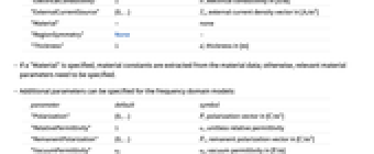
"Material"が指定されていると，材料データから材料定数が抽出される．それ以外の場合は関係がある材料パラメータを指定しなければならない．
周波数領域モデルには以下の追加的なパラメータを使うことができる．

パラメータ	デフォルト	シンボル
"Polarization"	{0,…}	，分極ベクトル，[ $TemplateBox[{InterpretationBox[, 1], {"C", , "/", , {"m", ^, 2}}, coulombs per meter squared, {{(, "Coulombs", )}, /, {(, {"Meters", ^, 2}, )}}}, QuantityTF]$ ]
"RelativePermittivity"	1	，無単位の比誘電率
"RemanentPolarization"	{0,…}	，残留分極ベクトル，[ $TemplateBox[{InterpretationBox[, 1], {"C", , "/", , {"m", ^, 2}}, coulombs per meter squared, {{(, "Coulombs", )}, /, {(, {"Meters", ^, 2}, )}}}, QuantityTF]$ ]
"VacuumPermittivity"		，真空の誘電率，[]

パラメータはどれも空間変数と従属変数に依存することがある．
独立変数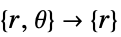の数が，，の次元とベクトル，，の長さを決定する．
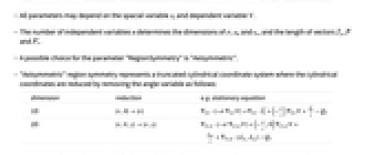
パラメータ"RegionSymmetry"の可能な選択肢には"Axisymmetric"がある．
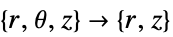
"Axisymmetric"領域対称性は，以下のように角変数を削除することで円筒座標が縮小される切頭円筒座標系を表す．
次元縮小例：定常方程式

1D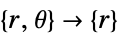

2D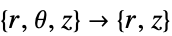
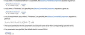
1Dで"CrossSectionalArea" が指定されていると，ElectricCurrentPDEComponent方程式は以下の形で与えられる．

2Dで"Thickness" が指定されていると，ElectricCurrentPDEComponent方程式は以下の形で与えられる．

1D軸対称性のケースで"Thickness" 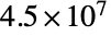が指定されていると，ElectricCurrentPDEComponent方程式は以下の形で与えられる．

パラメータについての入力指定は，対応する演算子項についてと厳密に同じである．
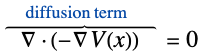
パラメータが指定されていない場合，デフォルトの電流PDEは以下のようになる．

ElectricCurrentPDEComponentが連想 pars で…,keyp_i…,p_iv_i,…として指定されたパラメータに依存するなら，パラメータはで置換される．

例題

すべて開くすべて閉じる

例 (4)

定常電流PDEモデルを定義する：

Wolfram Language code: ElectricCurrentPDEComponent[{V[x, y], {x, y}}, Entity["Element", "Copper"]]

記号時間依存電流PDEモデルを定義する：

Wolfram Language code:

ElectricCurrentPDEComponent[{V[t, x, y], t, {x, y}}, <|"ElectricalConductivity" -> σ, "RelativePermittivity" -> Subscript[ϵ, 𝓇], "VacuumPermittivity" -> Subscript[ϵ, 0], "Thickness" -> d|>]

記号周波電流PDEモデルを定義する：

Wolfram Language code:

ElectricCurrentPDEComponent[{V[x, y], ω, {x, y}}, <|"ElectricalConductivity" -> σ, "RelativePermittivity" -> Subscript[ϵ, 𝓇], "VacuumPermittivity" -> Subscript[ϵ, 0], "Thickness" -> d|>]

電気伝導率がのくびれた長方形のプレート内の電気スカラーポテンシャルについて解く：

Wolfram Language code:

Vfun = NDSolveValue[{ElectricCurrentPDEComponent[{V[x, y], {x, y}}, <|"ElectricalConductivity" -> 6*^7|>] == 0, ElectricPotentialCondition[y == -2, {V[x, y], {x, y}}, <|"ElectricPotential" -> 0|>], ElectricPotentialCondition[y == 2, {V[x, y], {x, y}}, <|"ElectricPotential" -> 1|>]}, V, {x, y}∈RegionUnion[Rectangle[{-1, -2}, {1, -0.3}], Rectangle[{-1, 0.3}, {1, 2}], Rectangle[{-0.3, -0.3}, {0.3, 0.3}]]];

電流密度ベクトルを計算する：

Wolfram Language code: Jfield = -6*^7 * Grad[Vfun[x, y], {x, y}];

電流密度ベクトルを可視化する：

Wolfram Language code:

VectorPlot[Jfield, {x, y}∈RegionUnion[Rectangle[{-1, -2}, {1, -0.3}], Rectangle[{-1, 0.3}, {1, 2}], Rectangle[{-0.3, -0.3}, {0.3, 0.3}]], AspectRatio -> Automatic]

スコープ (8)

記号定常電流PDEを定義する：

Wolfram Language code:

ElectricCurrentPDEComponent[{V[x, y], {x, y}}, <|"ElectricalConductivity" -> σ, "ExternalCurrentSource" -> {Jex[x, y], Jey[x, y]}, "CurrentSource" -> Subscript[Q, v], "Thickness" -> d|>]

定常電流PDEモデルを特定の材料について定義する：

Wolfram Language code: ElectricCurrentPDEComponent[{V[X, y], {x, y}}, <|"Material" -> Entity["Element", "Gold"]|>]

定常電流PDEを，導電率（単位 :[] ），外部電流密度（単位： [ $TemplateBox[{InterpretationBox[, 1], {"A", , "/", , {"m", ^, 2}}, amperes per meter squared, {{(, "Amperes", )}, /, {(, {"Meters", ^, 2}, )}}}, QuantityTF]$ ]）で指定する：

Wolfram Language code:

ElectricCurrentPDEComponent[{V[x, y], {x, y}}, <|"ElectricalConductivity" -> Quantity[4.5*^7, "Siemens"/"Meters"], "ExternalCurrentSource" -> {Quantity[10, "Amperes"/"Meters"^2], 0}|>]

特定の材料についての定常電流PDEモデルをアクティブにする(Activate)：

Wolfram Language code: Activate[ElectricCurrentPDEComponent[{V[X, y], {x, y}}, <|"Material" -> Entity["Element", "Gold"]|>]]

記号定常電流PDEを，伝導率，外部電流，電流源，厚みで定義する：

Wolfram Language code:

ElectricCurrentPDEComponent[{V[x, y], {x, y}}, <|"ElectricalConductivity" -> σ, "ExternalCurrentSource" -> {Jex[x, y], Jey[x, y]}, "CurrentSource" -> Subscript[Q, v], "Thickness" -> d|>]

記号2D軸対称定常電流PDEを定義する：

Wolfram Language code:

ElectricCurrentPDEComponent[{V[r, z], {r, z}}, <|"ElectricalConductivity" -> σ, "ExternalCurrentSource" -> {Jer[r, z], Jez[r, z]}, "CurrentSource" -> Subscript[Q, v], "RegionSymmetry" -> "Axisymmetric"|>]

3D周波電流PDEモデルを定義する：

Wolfram Language code:

ElectricCurrentPDEComponent[{V[x, y, z], ω, {x, y, z}}, <|"ElectricalConductivity" -> 4.5*^7, "RelativePermittivity" -> IdentityMatrix[3]|>]

3D時間依存電流PDEモデルを定義する：

Wolfram Language code: ElectricCurrentPDEComponent[{V[t, x, y, z], t, {x, y, z}}, <|"ElectricalConductivity" -> 4.5*^7|>]

アプリケーション (5)

2D定常解析 (1)

導電率がの3バー電気スイッチの電気スカラーポテンシャルについて解く：

Wolfram Language code:

Vfun = NDSolveValue[{ElectricCurrentPDEComponent[{V[x, y], {x, y}}, <|"ElectricalConductivity" -> 6*^7|>] == 0, ElectricPotentialCondition[y == -7.5, {V[x, y], {x, y}}, <|"ElectricPotential" -> 0|>], ElectricPotentialCondition[y == 7.5, {V[x, y], {x, y}}, <|"ElectricPotential" -> 5|>]}, V, {x, y}∈RegionUnion[Rectangle[{0, 2.5}, {10, 7.5}], Rectangle[{9, -2.5}, {10 + 9, 2.5}], Rectangle[{0, -7.5}, {10, -2.5}]]];

電流密度ベクトルを計算する：

Wolfram Language code: Jfield = -6*^7 * Grad[Vfun[x, y], {x, y}];

電流密度ベクトルを可視化する：

Wolfram Language code:

VectorPlot[Jfield, {x, y}∈RegionUnion[Rectangle[{0, 2.5}, {10, 7.5}], Rectangle[{9, -2.5}, {10 + 9, 2.5}], Rectangle[{0, -7.5}, {10, -2.5}]], AspectRatio -> Automatic]

3D定常解析 (3)

[]の直流電流(DC)で励起される銅線を上方境界における境界電流密度条件と下方境界におけるゼロ電位条件でモデル化する．

定常電流PDEモデルの変数とを設定する：

Wolfram Language code:

vars = {V[x, y, z], {x, y, z}};
pars = <|"Material" -> Entity["Element", "Copper"]|>;

方程式を設定する：

Wolfram Language code: op = ElectricCurrentPDEComponent[vars, pars];

下方境界における地電位を指定する：

Wolfram Language code: Subscript[Γ, ground] = ElectricPotentialCondition[z == 0, vars, pars, <|"ElectricPotential" -> 0|>];

上方境界における流入電流の流れを指定する：

Wolfram Language code: Subscript[Γ, source] = ElectricCurrentDensityValue[z == 0.01, vars, pars, <|"Current" -> 1|>];

円柱を定義する：

Wolfram Language code: Ω = Cylinder[{{0, 0, 0}, {0, 0, 0.01}}, 0.0005];

PDEを解く：

Wolfram Language code: Vfun = NDSolveValue[{op == Subscript[Γ, source], Subscript[Γ, ground]}, V, {x, y, z}∈Ω]

電位を可視化する：

Wolfram Language code:

Show[Graphics3D[{Opacity[0.2], Ω}, Boxed -> False], 
	SliceDensityPlot3D[Vfun[x, y, z], {x, y, z}∈Ω, ...]]

電位差 []のタングステンワイヤをモデル化する．定常電流偏微分方程式のモデル変数とを設定する：

Wolfram Language code:

vars = {V[x, y, z], {x, y, z}};
pars = <|"Material" -> Entity["Element", "Tungsten"]|>;

定常電流偏微分方程式を設定する：

Wolfram Language code: op = ElectricCurrentPDEComponent[vars, pars];

タングステンワイヤの半径は []で，ワイヤの幾何学形状はS字型である．幾何学パラメータを指定する：

Wolfram Language code:

L = 0.05;
r = 0.0025;
R = 0.0075;

シミュレーション領域：

Wolfram Language code: Ω = \!$\*Graphics3DBox[«5»]$;

左端境界では []の電位境界条件が適用され，右端境界ではゼロ電位条件が適用される．離散化領域の数値誤差を考慮して，許容値が両端に適用される．

ワイヤの両端に電位境界条件を設定する：

Wolfram Language code:

Subscript[Γ, potential] = {ElectricPotentialCondition[Abs[x] ≤ 0.01r && y^2 + z^2 ≤ r^2, vars, pars, <|"ElectricPotential" -> 0.2|>], ElectricPotentialCondition[Abs[y + r] ≤ 0.01r && (x - (L + 2R + r))^2 + z^2 ≤ r^2, vars, pars]};

偏微分方程式を解く：

Wolfram Language code: Vfun = NDSolveValue[{op == 0, Subscript[Γ, potential]}, V, {x, y, z}∈Ω]

電流密度ベクトルを計算する：

Wolfram Language code: Jfield = -QuantityMagnitude[pars["Material"]["ElectricalConductivity"]] * Grad[Vfun[x, y, z], {x, y, z}];

電流密度の大きさを可視化する：

Wolfram Language code:

SliceDensityPlot3D[Sqrt[Total[Jfield ^ 2]], {{"XStackedPlanes", 10}, {"YStackedPlanes", 12}, {"ZStackedPlanes", 3}}, {x, y, z}∈Ω, ...]

左境界に対して垂直な電流密度で励起され，右境界でゼロ電位境界条件を持つ銅スパイラルインダクタをモデル化する．

スパイラルインダクタの形状を定義する：

Wolfram Language code:

Ω = RegionUnion[Cuboid[{0, 0, 0}, {2, 1, 1}], Cuboid[{1, 1, 0}, {2, 8, 1}], Cuboid[{2, 7, 0}, {8, 8, 1}], Cuboid[{7, 7, 0}, {8, 0, 1}], Cuboid[{7, 0, 0}, {3, 1, 1}], Cuboid[{3, 1, 0}, {4, 6, 1}], Cuboid[{4, 6, 0}, {6, 5, 1}], Cuboid[{6, 5, 0}, {5, 2, 1}], Cuboid[{5, 2, 1}, {6, 3, 1.2}], Cuboid[{5, 2, 1.2}, {10, 3, 2.2}]]

定常電流偏微分モデル変数とを設定する：

Wolfram Language code:

vars = {V[x, y, z], {x, y, z}};
pars = <|"Material" -> Entity["Element", "Copper"]|>;

左境界に内向きの電流フローを指定する：

Wolfram Language code: Subscript[Γ, source] = ElectricCurrentDensityValue[x == 0, vars, pars, <|"NormalCurrentDensity" -> 10|>];

地位を指定する：

Wolfram Language code: Subscript[Γ, ground] = ElectricPotentialCondition[x == 10, vars, pars];

偏微分方程式を解く：

Wolfram Language code:

Vfun = NDSolveValue[{ElectricCurrentPDEComponent[vars, pars] == Subscript[Γ, source], Subscript[Γ, ground]}, V, {x, y, z}∈Ω]

電流密度ベクトルを計算する：

Wolfram Language code: Jfield = -QuantityMagnitude[pars["Material"]["ElectricalConductivity"]] * Grad[Vfun[x, y, z], {x, y, z}];

電流密度の大きさを可視化する：

Wolfram Language code:

SliceDensityPlot3D[Sqrt[Total[Jfield ^ 2]], {{"XStackedPlanes", 10}, {"YStackedPlanes", 10}, {"ZStackedPlanes", 5}}, {x, y, z}∈Ω, ...]

周波数解析 (1)

[]の交流電流(AC)で励起される円筒形コンデンサの誘電材料を，コンデンサの電極を表す上方境界の電流密度条件と下方境界の電位ゼロ状態でモデル化する．

周波電流PDEモデル変数を設定する：

Wolfram Language code: vars = {V[x, y, z], ω, {x, y, z}};

周波数と周期を定義する：

Wolfram Language code:

f0 = 60;
T0 = 1 / f0;

領域を設定する：

Wolfram Language code:

r0 = 0.01;
h = 0.001;
Ω = Cylinder[{{0, 0, 0}, {0, 0, h}}, r0];

導電率と比誘電率を指定する：

Wolfram Language code: pars = <|"ElectricalConductivity" -> 1*^-8, "RelativePermittivity" -> 2|>;

下方境界における地電位を指定する：

Wolfram Language code: Subscript[Γ, ground] = ElectricPotentialCondition[z == 0, vars, pars];

上方境界における流入電流を指定する：

Wolfram Language code: Subscript[Γ, current] = ElectricCurrentDensityValue[z == h, vars, pars, <|"Current" -> 1*^-7|>];

方程式を設定する：

Wolfram Language code: op = ElectricCurrentPDEComponent[vars, pars];

調和PDEを []について解く：

Wolfram Language code: Vfun = NDSolveValue[{(op /. {ω -> 2 Pi f0}) == Subscript[Γ, current], Subscript[Γ, ground]}, V, {x, y, z}∈Ω]

上方境界の電圧を時間領域に変換する：

Wolfram Language code: Vlist = Table[{t, Re[Vfun[0, 0, h] * Exp[I ω t] /. {ω -> 2 Pi f0}]}, {t, 0, 3 * T0, T0 / 100}];

コンデンサの上部プレートの電圧を可視化する：

Wolfram Language code: ListLinePlot[Vlist]

考えられる問題 (2)

記号計算の場合は，"ElectricalConductivity"，"VacuumPermittivity"あるいは"RelativePermittivity"のパラメータが行列として与えられなければならない：

Wolfram Language code:

ElectricCurrentPDEComponent[{V[x, y], ω, {x, y}}, <|"ElectricalConductivity" -> σ * IdentityMatrix[2], "VacuumPermittivity" -> Subscript[ϵ, 0], "RelativePermittivity" -> {{Subscript[ϵ, r11], 0}, {0, Subscript[ϵ, r12]}}|>]//Activate

数値計算の場合は，"ElectricalConductivity"，"VacuumPermittivity"あるいは"RelativePermittivity"のパラメータが，適切な次元の行列に自動的に変換される：

Wolfram Language code: ElectricCurrentPDEComponent[{V[x, y], {x, y}}, <|"ElectricalConductivity" -> 10|>]

自動変換は記号入力については行われない：

Wolfram Language code: ElectricCurrentPDEComponent[{V[x], {x}}, <|"ElectricalConductivity" -> σ|>]

適切な次元の行列を与えないとエラーになる：

Wolfram Language code: %//Activate

周波数領域モデルについては，"Material"が指定されている場合に材料パラメータを使うことはできない：

Wolfram Language code: ElectricCurrentPDEComponent[{V[x, y], ω, {x, y}}, <|"Material" -> Entity["Element", "Copper"]|>]

Top

その他のラーニングリソース

テクニカルサポート

データサイエンス，金融，ビジネス

工学

科学とテクノロジー

教育のためのテクノロジー

教育イニシアチブ

使い始める

Grow Your Skills

Wolframと繋がる

大人用の教育プログラム

若者のための教育プログラム

読む

ElectricCurrentPDEComponent

詳細

例題

例 (4)

スコープ (8)

アプリケーション (5)

2D定常解析 (1)

3D定常解析 (3)

周波数解析 (1)

考えられる問題 (2)

テキスト

CMS

APA

BibTeX

BibLaTeX

次元	縮小	例：定常方程式
1D
2D

ElectricCurrentPDEComponent

詳細

例題

例 (4)

スコープ (8)

アプリケーション (5)

2D定常解析 (1)

3D定常解析 (3)

周波数解析 (1)

考えられる問題 (2)

関連項目

テクニカルノート

関連するガイド

履歴

テキスト

CMS

APA

BibTeX

BibLaTeX