Wolfram 语言与系统参考资料中心

ElectricCurrentPDEComponent

ElectricCurrentPDEComponent[vars,pars]

生成带有变量 vars 和参数 pars 的电流偏微分方程项.

更多信息

ElectricCurrentPDEComponent 通常用于生成具有模型变量 vars 和模型参数 pars 的电流连续性方程.
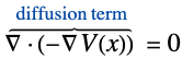
ElectricCurrentPDEComponent 返回一组微分算子之和，用作偏微分方程的一部分：

ElectricCurrentPDEComponent 创建用于稳态、频率和参数分析的偏微分方程项.
ElectricCurrentPDEComponent 模拟导电材料中由直流或交流电流产生的电场，在此情况下可忽略磁效应和感应效应.
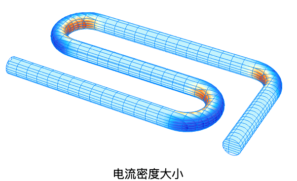
ElectricCurrentPDEComponent 的结果可用于计算电流密度的大小. »

ElectricCurrentPDEComponent 模拟稳态或谐波电场，其中电标量电势 [] 为因变量， [] 为自变量.
稳态变量 vars 为 vars={V[x₁,…,x_n],{x₁,…,x_n}}.
时间依赖变量 vars are vars={V[t,x₁,…,x_n],t,{x₁,…,x_n}}.
与频率相关的变量 vars 为 vars={V[x₁,…,x_n],ω,{x₁,…,x_n}}.
电流连续性方程为，其中体电荷密度，单位为 [ $TemplateBox[{InterpretationBox[, 1], {"C", , "/", , {"m", ^, 3}}, coulombs per meter cubed, {{(, "Coulombs", )}, /, {(, {"Meters", ^, 3}, )}}}, QuantityTF]$ ]，时间变量，单位为 []，电流密度向量，单位为 [ $TemplateBox[{InterpretationBox[, 1], {"A", , "/", , {"m", ^, 2}}, amperes per meter squared, {{(, "Amperes", )}, /, {(, {"Meters", ^, 2}, )}}}, QuantityTF]$ ].
本构材料模型方程，即欧姆定律，为，其中 [] 为导电率， [] 为电场强度，且有 .
ElectricCurrentPDEComponent 提供了一个稳态电流模型，其中是一个外部产生的电流密度矢量, 单位为 [ $TemplateBox[{InterpretationBox[, 1], {"A", , "/", , {"m", ^, 2}}, amperes per meter squared, {{(, "Amperes", )}, /, {(, {"Meters", ^, 2}, )}}}, QuantityTF]$ ]，代表电流源，单位为 [ $TemplateBox[{InterpretationBox[, 1], {"A", , "/", , {"m", ^, 3}}, amperes per meter cubed, {{(, "Amperes", )}, /, {(, {"Meters", ^, 3}, )}}}, QuantityTF]$ ]：

ElectricCurrentPDEComponent 提供了一个时域模型，其中时间变量为 []，真空介电常数为 [] 和相对介电常数为 []：

ElectricCurrentPDEComponent 提供了一个频域模型，其中 [] 为真空介电常数， [ $TemplateBox[{InterpretationBox[, 1], {"C", , "/", , {"m", ^, 2}}, coulombs per meter squared, {{(, "Coulombs", )}, /, {(, {"Meters", ^, 2}, )}}}, QuantityTF]$ ] 为极化向量， [] 为角频率，为虚数单位：

对于线性材料，频率域模型可以简化为：

是无量纲的相对介电常数.
可以是各向同性、正交各向异性，或完全各向异性.
对于电流模型，隐含的默认边界条件是 0 ElectricCurrentDensityValue.
电流模型中各项的单位是 [ $TemplateBox[{InterpretationBox[, 1], {"A", , "/", , {"m", ^, 3}}, amperes per meter cubed, {{(, "Amperes", )}, /, {(, {"Meters", ^, 3}, )}}}, QuantityTF]$ ].
可以给出以下参数 pars：

参数	默认值	符号
"CrossSectionalArea"	1	横截面积，单位为 [ $TemplateBox[{InterpretationBox[, 1], {{"m", ^, 2}}, meters squared, {"Meters", ^, 2}}, QuantityTF]$ ]
"CurrentSource"	0	电流源，单位为 [ $TemplateBox[{InterpretationBox[, 1], {"A", , "/", , {"m", ^, 3}}, amperes per meter cubed, {{(, "Amperes", )}, /, {(, {"Meters", ^, 3}, )}}}, QuantityTF]$ ]
"ElectricalConductivity"	1	，单位为 []
"ExternalCurrentSource"	{0,…}	外部电流密度矢量，单位为 [ $TemplateBox[{InterpretationBox[, 1], {"A", , "/", , {"m", ^, 2}}, amperes per meter squared, {{(, "Amperes", )}, /, {(, {"Meters", ^, 2}, )}}}, QuantityTF]$ ]
"Material"	-	无
"RegionSymmetry"	None
"Thickness"	1	厚度，单位为 []

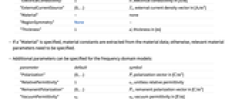
如果指定了 "Material"，则相关的材料常数将从材料数据中提取；否则，需要明确指定相关的材料参数.
对于频域模型，可以指定额外的参数：

参数	默认值	符号
"Polarization"	{0,…}	极化矢量，单位为 [ $TemplateBox[{InterpretationBox[, 1], {"C", , "/", , {"m", ^, 2}}, coulombs per meter squared, {{(, "Coulombs", )}, /, {(, {"Meters", ^, 2}, )}}}, QuantityTF]$ ]
"RelativePermittivity"	1	，无量纲的相对介电常数
"RemanentPolarization"	{0,…}	残余极化矢量，单位为 [ $TemplateBox[{InterpretationBox[, 1], {"C", , "/", , {"m", ^, 2}}, coulombs per meter squared, {{(, "Coulombs", )}, /, {(, {"Meters", ^, 2}, )}}}, QuantityTF]$ ]
"VacuumPermittivity"		真空介电常数，单位为 []

所有参数可能取决于空间变量和因变量 .
自变量的数量决定了、和的维度，以及矢量、和的长度.
参数 "RegionSymmetry" 的可能选择是 "Axisymmetric".
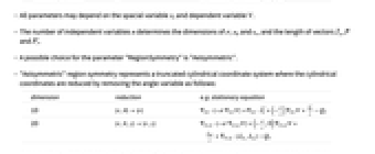
"Axisymmetric" 区域对称性表示一个截断的柱坐标系，其中柱坐标通过移除角变量被简化，具体如下：
维度简化 例如：稳态方程

1D

2D
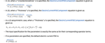
在一维情况下，如果指定了 "CrossSectionalArea" ，ElectricCurrentPDEComponent 方程如下：

在一维情况下，如果指定了 "Thickness" ，ElectricCurrentPDEComponent 方程如下：

在一维轴对称情况下，当指定 "Thickness" 时，ElectricCurrentPDEComponent 方程如下：

参数的输入规范与其相应的运算符项完全相同.
如果不指定参数，则默认电流偏微分方程为：

如果 ElectricCurrentPDEComponent 取决于在关联 pars 中指定为 …,keyp_i…,p_iv_i,… 的参数，则参数将替换为 .

范例

打开所有单元关闭所有单元

基本范例 (4)

定义稳态电流偏微分方程模型：

Wolfram Language code: ElectricCurrentPDEComponent[{V[x, y], {x, y}}, Entity["Element", "Copper"]]

定义符号时间依赖电流偏微分方程模型：

Wolfram Language code:

ElectricCurrentPDEComponent[{V[t, x, y], t, {x, y}}, <|"ElectricalConductivity" -> σ, "RelativePermittivity" -> Subscript[ϵ, 𝓇], "VacuumPermittivity" -> Subscript[ϵ, 0], "Thickness" -> d|>]

定义符号频率电流偏微分方程模型：

Wolfram Language code:

ElectricCurrentPDEComponent[{V[x, y], ω, {x, y}}, <|"ElectricalConductivity" -> σ, "RelativePermittivity" -> Subscript[ϵ, 𝓇], "VacuumPermittivity" -> Subscript[ϵ, 0], "Thickness" -> d|>]

求解电导率为的收缩矩形板的标量电势：

Wolfram Language code:

Vfun = NDSolveValue[{ElectricCurrentPDEComponent[{V[x, y], {x, y}}, <|"ElectricalConductivity" -> 6*^7|>] == 0, ElectricPotentialCondition[y == -2, {V[x, y], {x, y}}, <|"ElectricPotential" -> 0|>], ElectricPotentialCondition[y == 2, {V[x, y], {x, y}}, <|"ElectricPotential" -> 1|>]}, V, {x, y}∈RegionUnion[Rectangle[{-1, -2}, {1, -0.3}], Rectangle[{-1, 0.3}, {1, 2}], Rectangle[{-0.3, -0.3}, {0.3, 0.3}]]];

计算电流密度矢量：

Wolfram Language code: Jfield = -6*^7 * Grad[Vfun[x, y], {x, y}];

可视化电流密度矢量：

Wolfram Language code:

VectorPlot[Jfield, {x, y}∈RegionUnion[Rectangle[{-1, -2}, {1, -0.3}], Rectangle[{-1, 0.3}, {1, 2}], Rectangle[{-0.3, -0.3}, {0.3, 0.3}]], AspectRatio -> Automatic]

范围 (8)

定义符号稳态电流偏微分方程模型：

Wolfram Language code:

ElectricCurrentPDEComponent[{V[x, y], {x, y}}, <|"ElectricalConductivity" -> σ, "ExternalCurrentSource" -> {Jex[x, y], Jey[x, y]}, "CurrentSource" -> Subscript[Q, v], "Thickness" -> d|>]

对于特定材料，定义稳态电流的偏微分方程模型：

Wolfram Language code: ElectricCurrentPDEComponent[{V[X, y], {x, y}}, <|"Material" -> Entity["Element", "Gold"]|>]

指定一个稳态电流的偏微分方程，其中电导率（单位为 []），外部电流密度（单位为[ $TemplateBox[{InterpretationBox[, 1], {"A", , "/", , {"m", ^, 2}}, amperes per meter squared, {{(, "Amperes", )}, /, {(, {"Meters", ^, 2}, )}}}, QuantityTF]$ ]）：

Wolfram Language code:

ElectricCurrentPDEComponent[{V[x, y], {x, y}}, <|"ElectricalConductivity" -> Quantity[4.5*^7, "Siemens"/"Meters"], "ExternalCurrentSource" -> {Quantity[10, "Amperes"/"Meters"^2], 0}|>]

用 Activate 激活一个特定材料的稳态电流偏微分方程模型：

Wolfram Language code: Activate[ElectricCurrentPDEComponent[{V[X, y], {x, y}}, <|"Material" -> Entity["Element", "Gold"]|>]]

通过电导率、外部电流、电流源和厚度，定义一个符号稳态电流偏微分方程：

Wolfram Language code:

ElectricCurrentPDEComponent[{V[x, y], {x, y}}, <|"ElectricalConductivity" -> σ, "ExternalCurrentSource" -> {Jex[x, y], Jey[x, y]}, "CurrentSource" -> Subscript[Q, v], "Thickness" -> d|>]

定义符号二维轴对称稳态电流偏微分方程：

Wolfram Language code:

ElectricCurrentPDEComponent[{V[r, z], {r, z}}, <|"ElectricalConductivity" -> σ, "ExternalCurrentSource" -> {Jer[r, z], Jez[r, z]}, "CurrentSource" -> Subscript[Q, v], "RegionSymmetry" -> "Axisymmetric"|>]

定义三维频率电流偏微分方程模型：

Wolfram Language code:

ElectricCurrentPDEComponent[{V[x, y, z], ω, {x, y, z}}, <|"ElectricalConductivity" -> 4.5*^7, "RelativePermittivity" -> IdentityMatrix[3]|>]

定义三维时间依赖电流偏微分方程模型：

Wolfram Language code: ElectricCurrentPDEComponent[{V[t, x, y, z], t, {x, y, z}}, <|"ElectricalConductivity" -> 4.5*^7|>]

应用 (5)

二维稳态分析 (1)

求解一个 3 杆电开关的电势标量，已知其电导率为：

Wolfram Language code:

Vfun = NDSolveValue[{ElectricCurrentPDEComponent[{V[x, y], {x, y}}, <|"ElectricalConductivity" -> 6*^7|>] == 0, ElectricPotentialCondition[y == -7.5, {V[x, y], {x, y}}, <|"ElectricPotential" -> 0|>], ElectricPotentialCondition[y == 7.5, {V[x, y], {x, y}}, <|"ElectricPotential" -> 5|>]}, V, {x, y}∈RegionUnion[Rectangle[{0, 2.5}, {10, 7.5}], Rectangle[{9, -2.5}, {10 + 9, 2.5}], Rectangle[{0, -7.5}, {10, -2.5}]]];

计算电流密度矢量：

Wolfram Language code: Jfield = -6*^7 * Grad[Vfun[x, y], {x, y}];

可视化电流密度矢量：

Wolfram Language code:

VectorPlot[Jfield, {x, y}∈RegionUnion[Rectangle[{0, 2.5}, {10, 7.5}], Rectangle[{9, -2.5}, {10 + 9, 2.5}], Rectangle[{0, -7.5}, {10, -2.5}]], AspectRatio -> Automatic]

三维稳态分析 (3)

对用 [] 的直流电 (DC) 激励的铜线进行建模，其上边界为电流密度边界条件，下边界为零电势条件.

设置稳态电流偏微分方程模型变量和：

Wolfram Language code:

vars = {V[x, y, z], {x, y, z}};
pars = <|"Material" -> Entity["Element", "Copper"]|>;

设定方程：

Wolfram Language code: op = ElectricCurrentPDEComponent[vars, pars];

指定下边界处的接地电位：

Wolfram Language code: Subscript[Γ, ground] = ElectricPotentialCondition[z == 0, vars, pars, <|"ElectricPotential" -> 0|>];

指定上边界处的内向电流：

Wolfram Language code: Subscript[Γ, source] = ElectricCurrentDensityValue[z == 0.01, vars, pars, <|"Current" -> 1|>];

定义圆柱体：

Wolfram Language code: Ω = Cylinder[{{0, 0, 0}, {0, 0, 0.01}}, 0.0005];

求解偏微分方程：

Wolfram Language code: Vfun = NDSolveValue[{op == Subscript[Γ, source], Subscript[Γ, ground]}, V, {x, y, z}∈Ω]

可视化电势：

Wolfram Language code:

Show[Graphics3D[{Opacity[0.2], Ω}, Boxed -> False], 
	SliceDensityPlot3D[Vfun[x, y, z], {x, y, z}∈Ω, ...]]

对电位差为 []的钨丝进行建模. 设置平稳电流偏微分方程模型变量和：

Wolfram Language code:

vars = {V[x, y, z], {x, y, z}};
pars = <|"Material" -> Entity["Element", "Tungsten"]|>;

设置稳态电流偏微分方程：

Wolfram Language code: op = ElectricCurrentPDEComponent[vars, pars];

钨丝的半径为 []，几何形状为 S 形. 指定几何参数：

Wolfram Language code:

L = 0.05;
r = 0.0025;
R = 0.0075;

模拟域：

Wolfram Language code: Ω = \!$\*Graphics3DBox[«5»]$;

在左端边界应用电势边界条件 []，在右端边界处应用零电势条件. 在两端各留出的容差，以解决离散域中的数值误差.

设置钨丝两端的电势边界条件：

Wolfram Language code:

Subscript[Γ, potential] = {ElectricPotentialCondition[Abs[x] ≤ 0.01r && y^2 + z^2 ≤ r^2, vars, pars, <|"ElectricPotential" -> 0.2|>], ElectricPotentialCondition[Abs[y + r] ≤ 0.01r && (x - (L + 2R + r))^2 + z^2 ≤ r^2, vars, pars]};

求解偏微分方程：

Wolfram Language code: Vfun = NDSolveValue[{op == 0, Subscript[Γ, potential]}, V, {x, y, z}∈Ω]

计算电流密度矢量：

Wolfram Language code: Jfield = -QuantityMagnitude[pars["Material"]["ElectricalConductivity"]] * Grad[Vfun[x, y, z], {x, y, z}];

可视化电流密度大小：

Wolfram Language code:

SliceDensityPlot3D[Sqrt[Total[Jfield ^ 2]], {{"XStackedPlanes", 10}, {"YStackedPlanes", 12}, {"ZStackedPlanes", 3}}, {x, y, z}∈Ω, ...]

建立一个铜螺旋电感器模型，该电感器在左边界以法线电流密度激励，右边界的电动势边界条件为零.

定义螺旋电感器的几何属性：

Wolfram Language code:

Ω = RegionUnion[Cuboid[{0, 0, 0}, {2, 1, 1}], Cuboid[{1, 1, 0}, {2, 8, 1}], Cuboid[{2, 7, 0}, {8, 8, 1}], Cuboid[{7, 7, 0}, {8, 0, 1}], Cuboid[{7, 0, 0}, {3, 1, 1}], Cuboid[{3, 1, 0}, {4, 6, 1}], Cuboid[{4, 6, 0}, {6, 5, 1}], Cuboid[{6, 5, 0}, {5, 2, 1}], Cuboid[{5, 2, 1}, {6, 3, 1.2}], Cuboid[{5, 2, 1.2}, {10, 3, 2.2}]]

设置静态电流偏微分模型变量和：

Wolfram Language code:

vars = {V[x, y, z], {x, y, z}};
pars = <|"Material" -> Entity["Element", "Copper"]|>;

在左边界指定内向电流：

Wolfram Language code: Subscript[Γ, source] = ElectricCurrentDensityValue[x == 0, vars, pars, <|"NormalCurrentDensity" -> 10|>];

指定接地电位：

Wolfram Language code: Subscript[Γ, ground] = ElectricPotentialCondition[x == 10, vars, pars];

求解偏微分方程：

Wolfram Language code:

Vfun = NDSolveValue[{ElectricCurrentPDEComponent[vars, pars] == Subscript[Γ, source], Subscript[Γ, ground]}, V, {x, y, z}∈Ω]

计算电流密度矢量：

Wolfram Language code: Jfield = -QuantityMagnitude[pars["Material"]["ElectricalConductivity"]] * Grad[Vfun[x, y, z], {x, y, z}];

可视化电流密度大小：

Wolfram Language code:

SliceDensityPlot3D[Sqrt[Total[Jfield ^ 2]], {{"XStackedPlanes", 10}, {"YStackedPlanes", 10}, {"ZStackedPlanes", 5}}, {x, y, z}∈Ω, ...]

频率分析 (1)

对圆柱形电容器的介电材料进行建模，该电容器用 [] 的交流电 (AC) 激励，在上电极应用电流密度边界条件，在下边界应用零电势边界条件.

设置频率电流偏微分方程模型变量：

Wolfram Language code: vars = {V[x, y, z], ω, {x, y, z}};

定义频率和周期：

Wolfram Language code:

f0 = 60;
T0 = 1 / f0;

设置区域：

Wolfram Language code:

r0 = 0.01;
h = 0.001;
Ω = Cylinder[{{0, 0, 0}, {0, 0, h}}, r0];

指定电导率和相对介电常数：

Wolfram Language code: pars = <|"ElectricalConductivity" -> 1*^-8, "RelativePermittivity" -> 2|>;

指定下边界处的接地电位：

Wolfram Language code: Subscript[Γ, ground] = ElectricPotentialCondition[z == 0, vars, pars];

指定上边界处的内向电流：

Wolfram Language code: Subscript[Γ, current] = ElectricCurrentDensityValue[z == h, vars, pars, <|"Current" -> 1*^-7|>];

设定方程：

Wolfram Language code: op = ElectricCurrentPDEComponent[vars, pars];

求解 [] 时的谐波偏微分方程：

Wolfram Language code: Vfun = NDSolveValue[{(op /. {ω -> 2 Pi f0}) == Subscript[Γ, current], Subscript[Γ, ground]}, V, {x, y, z}∈Ω]

将上边界电压变换到时域：

Wolfram Language code: Vlist = Table[{t, Re[Vfun[0, 0, h] * Exp[I ω t] /. {ω -> 2 Pi f0}]}, {t, 0, 3 * T0, T0 / 100}];

可视化电容器上极板的电压：

Wolfram Language code: ListLinePlot[Vlist]

可能存在的问题 (2)

对于符号计算，"ElectricalConductivity"、"VacuumPermittivity" 或 "RelativePermittivity" 参数应该以矩阵形式给出：

Wolfram Language code:

ElectricCurrentPDEComponent[{V[x, y], ω, {x, y}}, <|"ElectricalConductivity" -> σ * IdentityMatrix[2], "VacuumPermittivity" -> Subscript[ϵ, 0], "RelativePermittivity" -> {{Subscript[ϵ, r11], 0}, {0, Subscript[ϵ, r12]}}|>]//Activate

对于数值，"ElectricalConductivity"、"VacuumPermittivity" 或 "RelativePermittivity" 参数自动转换为适当维度的矩阵：

Wolfram Language code: ElectricCurrentPDEComponent[{V[x, y], {x, y}}, <|"ElectricalConductivity" -> 10|>]

对于符号输入来说，这种自动转换是不可能的：

Wolfram Language code: ElectricCurrentPDEComponent[{V[x], {x}}, <|"ElectricalConductivity" -> σ|>]

不提供正确维度的矩阵将导致错误：

Wolfram Language code: %//Activate

对于频域模型，当指定 "Material" 时，材料参数不可用：

Wolfram Language code: ElectricCurrentPDEComponent[{V[x, y], ω, {x, y}}, <|"Material" -> Entity["Element", "Copper"]|>]

Top

更多学习资源

技术支持

数据科学、金融与商业

工程

科学与技术

教育科技

教育举措

开始

提高你的技能

与我们合作

成人教育计划

青少年教育计划

欢迎阅读

ElectricCurrentPDEComponent

更多信息

范例

基本范例 (4)

范围 (8)

应用 (5)

二维稳态分析 (1)

三维稳态分析 (3)

频率分析 (1)

可能存在的问题 (2)

文本

CMS

APA

BibTeX

BibLaTeX

维度	简化	例如：稳态方程
1D
2D

ElectricCurrentPDEComponent

更多信息

范例

基本范例 (4)

范围 (8)

应用 (5)

二维稳态分析 (1)

三维稳态分析 (3)

频率分析 (1)

可能存在的问题 (2)

参见

技术笔记

相关指南

历史

文本

CMS

APA

BibTeX

BibLaTeX