FluidFlowPDEComponent[vars,pars]
yields a flow PDE term with variables vars and parameters pars.


FluidFlowPDEComponent
FluidFlowPDEComponent[vars,pars]
yields a flow PDE term with variables vars and parameters pars.
Details
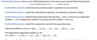
- FluidFlowPDEComponent models flow of viscous fluids subject to applied forces and constraints.
- FluidFlowPDEComponent returns a sum of differential operators to be used as a part of partial differential equations:
- FluidFlowPDEComponent models fluid flow phenomena with velocities
 ,
,  and
and  in units of [
![TemplateBox[{InterpretationBox[, 1], {"m", , "/", , "s"}, meters per second, {{(, "Meters", )}, /, {(, "Seconds", )}}}, QuantityTF] TemplateBox[{InterpretationBox[, 1], {"m", , "/", , "s"}, meters per second, {{(, "Meters", )}, /, {(, "Seconds", )}}}, QuantityTF]](Files/FluidFlowPDEComponent.en/5.png) ] as dependent variables,
] as dependent variables,  as independent variables in units of [
![TemplateBox[{InterpretationBox[, 1], "m", meters, "Meters"}, QuantityTF] TemplateBox[{InterpretationBox[, 1], "m", meters, "Meters"}, QuantityTF]](Files/FluidFlowPDEComponent.en/7.png) ] and time variable
] and time variable  in units of [
![TemplateBox[{InterpretationBox[, 1], "s", seconds, "Seconds"}, QuantityTF] TemplateBox[{InterpretationBox[, 1], "s", seconds, "Seconds"}, QuantityTF]](Files/FluidFlowPDEComponent.en/9.png) ].
]. - FluidFlowPDEComponent creates PDE components for stationary, time-dependent, parametric analysis.
- FluidFlowPDEComponent creates PDE components in two and three space dimensions.
- Stationary variables vars are vars={{u[x1,…,xn],v[x1,…,xn],…,p[x1,…,xn]},{x1,…,xn}}.
- Time-dependent or eigenmode variables vars are vars={{u[t,x1,…,xn],v[t,x1,…,xn],…,p[x1,…,xn]},t,{x1,…,xn}}.
- The equations for different analysis types that FluidFlowPDEComponent generates depend on the form of vars.
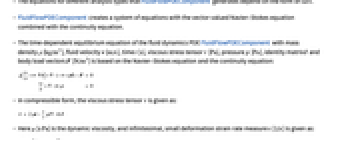
- FluidFlowPDEComponent creates a system of equations with the vector-valued Navier–Stokes equation combined with the continuity equation.
- The time-dependent equilibrium equation of the fluid dynamics PDE FluidFlowPDEComponent with mass density
 [
[![TemplateBox[{InterpretationBox[, 1], {"kg", , "/", , {"m", ^, 3}}, kilograms per meter cubed, {{(, "Kilograms", )}, /, {(, {"Meters", ^, 3}, )}}}, QuantityTF] TemplateBox[{InterpretationBox[, 1], {"kg", , "/", , {"m", ^, 3}}, kilograms per meter cubed, {{(, "Kilograms", )}, /, {(, {"Meters", ^, 3}, )}}}, QuantityTF]](Files/FluidFlowPDEComponent.en/12.png) ], fluid velocity
], fluid velocity  [
[![TemplateBox[{InterpretationBox[, 1], {"m", , "/", , "s"}, meters per second, {{(, "Meters", )}, /, {(, "Seconds", )}}}, QuantityTF] TemplateBox[{InterpretationBox[, 1], {"m", , "/", , "s"}, meters per second, {{(, "Meters", )}, /, {(, "Seconds", )}}}, QuantityTF]](Files/FluidFlowPDEComponent.en/14.png) ], time
], time  [
[![TemplateBox[{InterpretationBox[, 1], "s", seconds, "Seconds"}, QuantityTF] TemplateBox[{InterpretationBox[, 1], "s", seconds, "Seconds"}, QuantityTF]](Files/FluidFlowPDEComponent.en/16.png) ], viscous stress tensor
], viscous stress tensor  [
[![TemplateBox[{InterpretationBox[, 1], "Pa", pascals, "Pascals"}, QuantityTF] TemplateBox[{InterpretationBox[, 1], "Pa", pascals, "Pascals"}, QuantityTF]](Files/FluidFlowPDEComponent.en/18.png) ], pressure
], pressure  [
[![TemplateBox[{InterpretationBox[, 1], "Pa", pascals, "Pascals"}, QuantityTF] TemplateBox[{InterpretationBox[, 1], "Pa", pascals, "Pascals"}, QuantityTF]](Files/FluidFlowPDEComponent.en/20.png) ], identity matrix
], identity matrix  and body load vectors
  [
[![TemplateBox[{InterpretationBox[, 1], {"N", , "/", , {"m", ^, 3}}, newtons per meter cubed, {{(, "Newtons", )}, /, {(, {"Meters", ^, 3}, )}}}, QuantityTF] TemplateBox[{InterpretationBox[, 1], {"N", , "/", , {"m", ^, 3}}, newtons per meter cubed, {{(, "Newtons", )}, /, {(, {"Meters", ^, 3}, )}}}, QuantityTF]](Files/FluidFlowPDEComponent.en/23.png) ] is based on the Navier–Stokes equation and the continuity equation:
] is based on the Navier–Stokes equation and the continuity equation: - In compressible form, the viscous stress tensor
 is given as:
 - Here
 [
[![TemplateBox[{InterpretationBox[, 1], {"s", , "Pa"}, second pascals, {"Pascals", , "Seconds"}}, QuantityTF] TemplateBox[{InterpretationBox[, 1], {"s", , "Pa"}, second pascals, {"Pascals", , "Seconds"}}, QuantityTF]](Files/FluidFlowPDEComponent.en/28.png) ] is the dynamic viscosity, and infinitesimal, small deformation strain rate measure
] is the dynamic viscosity, and infinitesimal, small deformation strain rate measure  [1/
[1/![TemplateBox[{InterpretationBox[, 1], "s", seconds, "Seconds"}, QuantityTF] TemplateBox[{InterpretationBox[, 1], "s", seconds, "Seconds"}, QuantityTF]](Files/FluidFlowPDEComponent.en/30.png) ] is given as:
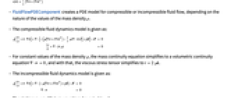
] is given as: - FluidFlowPDEComponent creates a PDE model for compressible or incompressible fluid flow, depending on the nature of the values of the mass density
 .
. - The compressible fluid dynamics model is given as:
- For constant values of the mass density
 , the mass continuity equation simplifies to a volumetric continuity equation
  , and with that, the viscous stress tensor simplifies to
  .
. - The incompressible fluid dynamics model is given as:
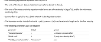
- The stationary equilibrium equations have
 .
. - The units of the Navier–Stokes model terms are a force density in [
![TemplateBox[{InterpretationBox[, 1], {"N", , "/", , {"m", ^, 3}}, newtons per meter cubed, {{(, "Newtons", )}, /, {(, {"Meters", ^, 3}, )}}}, QuantityTF] TemplateBox[{InterpretationBox[, 1], {"N", , "/", , {"m", ^, 3}}, newtons per meter cubed, {{(, "Newtons", )}, /, {(, {"Meters", ^, 3}, )}}}, QuantityTF]](Files/FluidFlowPDEComponent.en/39.png) ].
]. - The units of the mass continuity equation model terms are a force density in [
![TemplateBox[{InterpretationBox[, 1], {"kg", , "/(", , {"m", ^, 3}, , "s", , ")"}, kilograms per meter cubed second, {{(, "Kilograms", )}, /, {(, {{"Meters", ^, 3}, , "Seconds"}, )}}}, QuantityTF] TemplateBox[{InterpretationBox[, 1], {"kg", , "/(", , {"m", ^, 3}, , "s", , ")"}, kilograms per meter cubed second, {{(, "Kilograms", )}, /, {(, {{"Meters", ^, 3}, , "Seconds"}, )}}}, QuantityTF]](Files/FluidFlowPDEComponent.en/40.png) ], and for the volumetric continuity [1/
], and for the volumetric continuity [1/![TemplateBox[{InterpretationBox[, 1], "s", seconds, "Seconds"}, QuantityTF] TemplateBox[{InterpretationBox[, 1], "s", seconds, "Seconds"}, QuantityTF]](Files/FluidFlowPDEComponent.en/41.png) ].
]. - Laminar flow is typical for
 , where
  is the Reynolds number.
 - The Reynolds number
 is defined as
  , where
  [
[![TemplateBox[{InterpretationBox[, 1], "m", meters, "Meters"}, QuantityTF] TemplateBox[{InterpretationBox[, 1], "m", meters, "Meters"}, QuantityTF]](Files/FluidFlowPDEComponent.en/47.png) ] is a characteristic length and
] is a characteristic length and  the flow velocity.
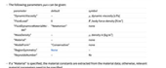
 - The following parameters pars can be given:
-
parameter default symbol "DynamicViscosity" -  , dynamic viscosity [
![TemplateBox[{InterpretationBox[, 1], {"s", , "Pa"}, second pascals, {"Pascals", , "Seconds"}}, QuantityTF] TemplateBox[{InterpretationBox[, 1], {"s", , "Pa"}, second pascals, {"Pascals", , "Seconds"}}, QuantityTF]](Files/FluidFlowPDEComponent.en/50.png) ]
]
"FluidLoad" 0  , body force density [
![TemplateBox[{InterpretationBox[, 1], {"N", , "/", , {"m", ^, 3}}, newtons per meter cubed, {{(, "Newtons", )}, /, {(, {"Meters", ^, 3}, )}}}, QuantityTF] TemplateBox[{InterpretationBox[, 1], {"N", , "/", , {"m", ^, 3}}, newtons per meter cubed, {{(, "Newtons", )}, /, {(, {"Meters", ^, 3}, )}}}, QuantityTF]](Files/FluidFlowPDEComponent.en/52.png) ]
]
"FluidDynamicsMaterialModel" "Newtonian" none "MassDensity" -  , density in [
![TemplateBox[{InterpretationBox[, 1], {"kg", , "/", , {"m", ^, 3}}, kilograms per meter cubed, {{(, "Kilograms", )}, /, {(, {"Meters", ^, 3}, )}}}, QuantityTF] TemplateBox[{InterpretationBox[, 1], {"kg", , "/", , {"m", ^, 3}}, kilograms per meter cubed, {{(, "Kilograms", )}, /, {(, {"Meters", ^, 3}, )}}}, QuantityTF]](Files/FluidFlowPDEComponent.en/54.png) ]
]
"Material" - none "ModelForm" "Conservative" none "RegionSymmetry" None - "ReynoldsNumber" - 
- If a "Material" is specified, the material constants are extracted from the material data; otherwise, relevant material parameters need to be specified.
- Instead of material parameters, a Reynolds number
 can be specified:
 - "RegionSymmetry"->"Axisymmetric" uses a truncated cylindrical coordinate system and assumes
 in the
  direction and pressure
  and velocity components
  and
and  independent of
  .
. - The axis of symmetry is the
 axis.
axis. - The default material model is a Newtonian flow model.
- Alternate material models can be specified by setting the "FluidDynamicsMaterialModel" key in parameters pars.
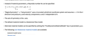
- The following non-Newtonian material models are available:
-
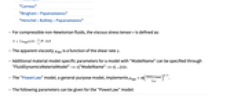
material model name "PowerLaw" "Carreau" "Bingham-Papanastasiou" "Herschel-Bulkley-Papanastasiou" - For compressible non-Newtonian fluids, the viscous stress tensor
 is defined as:
 - The apparent viscosity
 is a function of the shear rate
  .
. - Additional material model-specific parameters for a model with "ModelName" can be specified through "FluidDynamicsMaterialModel"-><|"ModelName"-><|...|>|>.
- The "PowerLaw" model, a general-purpose model, implements
 .
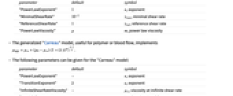
. - The following parameters can be given for the "PowerLaw" model:
-
parameter default symbol "PowerLawExponent" 
 , exponent
"MinimalShearRate" 
 , minimal shear rate
"ReferenceShearRate" 
 , reference shear rate
"PowerLawViscosity" 
 , power law viscosity
 - The generalized "Carreau" model, useful for polymer or blood flow, implements
 .
. - The following parameters can be given for the "Carreau" model:
-
parameter default symbol "PowerLawExponent" 
 , exponent
"TransitionExponent" 2  , exponent
"InfiniteShearRateViscosity" 
 , viscosity at inifinite shear rate
"Lambda" 
 , relaxation time [
![TemplateBox[{InterpretationBox[, 1], "s", seconds, "Seconds"}, QuantityTF] TemplateBox[{InterpretationBox[, 1], "s", seconds, "Seconds"}, QuantityTF]](Files/FluidFlowPDEComponent.en/86.png) ]
]"ZeroShearRateViscosity" 
 , viscosity at zero shear rate
 - The "Carreau" model can also be used for a Cross model where
 with
with  .
. - The "Bingham-Papanastasiou" model, useful for viscoplastic material, implements
 .
. - The following parameters can be given for the "Bingham-Papanastasiou" model:
-
parameter default symbol "PlasticViscosity" 
 , plastic viscosity
"YieldStress" 
 , yield stress
"ShearRateFactor" 
 , shear rate factor
 - The "Herschel-Bulkley-Papanastasiou" model, a mixture of a "PowerLaw" and "Bingham-Papanastasiou" model, implements
 . The model uses a power law to compute the plastic viscosity
  of the Bingham–Papanastasiou model, and parameters for both models can be set.
 - A custom apparent viscosity function fun can be specified as "FluidDynamicsMaterialModel"-><|"Custom"-><|"ApparentViscosityFunction"->fun|>|>.
- A custom apparent viscosity function fun has a function signature fun[name_,vars_,pars_,data__].
- Custom viscous stress tensor functions fun can be specified as "FluidDynamicsMaterialModel"->fun.
- A custom viscous stress tensor function fun has a function signature fun[vars_,pars_,data__].
- Non-isothermal flow can be modeled through the Boussinesq approximation.
- FluidFlowPDEComponent uses "SIBase" units. The geometry has to be in the same units as the PDE.
- If the FluidFlowPDEComponent depends on parameters
 that are specified in the association pars as …,keypi…,pivi,…, the parameters
  are replaced with
  .
.
Examples
open all close allBasic Examples (4)
Scope (10)
2D (4)
Define a flow PDE model for a specific material:
Specify a flow PDE with a dynamic viscosity of ![]() and a mass density of
and a mass density of ![]() :
:
Activate a flow PDE model for a specific material:
Specify a symbolic stationary fluid dynamics PDE in two dimensions with a dynamic viscosity of ![]() and a mass density of
and a mass density of ![]() :
:
2D Axisymmetric (1)
3D (1)
Time Dependent (3)
Applications (5)
Stationary Analysis (1)
Non-Newtonian Flow (1)
Compute the fluid flow of a non-Newtonian fluid in an opening channel by using the power law fluid flow model.
Set up variables, flow parameters and the non-Newtonian power law for parameters for the exponent and power law viscosity:
Solve the PDE with an inflow profile given as {1/2,0} and with the outflow pressure set to 0. The walls are set up as no-slip walls:
Visualize the velocity in the region:
Plot the flow profile from the middle of the channel to the top scaled to 1:
Time-Dependent Analysis (1)
Solve a time-dependent driven cavity problem.
Create and visualize an auxiliary function to ramp up the flow speed on top of the box:
Set up the boundary conditions:
Set up the initial conditions:
Monitor the solution process and measure the time it takes to solve the PDE:
Visualize rasterized frames of the velocity field for various times:
Axisymmetric Flow (2)
Compute the fluid flow in a narrowing cylindrical pipe driven by a parabolic inflow. Set up the axisymmetric domain:
Set up the boundary conditions:
Visualize the velocity of the solution:
Plot the pressure in 3D for part of the pipe:
Compute the velocity profile for time-dependent axisymmetric flow driven by a pressure gradient. Set up the domain:
Set up the boundary conditions with a prescribed pressure gradient:
Solve the equations and measure the time it takes:
Tech Notes
Related Guides
Text
Wolfram Research (2024), FluidFlowPDEComponent, Wolfram Language function, https://reference.wolfram.com/language/ref/FluidFlowPDEComponent.html (updated 2025).
CMS
Wolfram Language. 2024. "FluidFlowPDEComponent." Wolfram Language & System Documentation Center. Wolfram Research. Last Modified 2025. https://reference.wolfram.com/language/ref/FluidFlowPDEComponent.html.
APA
Wolfram Language. (2024). FluidFlowPDEComponent. Wolfram Language & System Documentation Center. Retrieved from https://reference.wolfram.com/language/ref/FluidFlowPDEComponent.html
BibTeX
@misc{reference.wolfram_2025_fluidflowpdecomponent, author="Wolfram Research", title="{FluidFlowPDEComponent}", year="2025", howpublished="\url{https://reference.wolfram.com/language/ref/FluidFlowPDEComponent.html}", note=[Accessed: 05-May-2026]}
BibLaTeX
@online{reference.wolfram_2025_fluidflowpdecomponent, organization={Wolfram Research}, title={FluidFlowPDEComponent}, year={2025}, url={https://reference.wolfram.com/language/ref/FluidFlowPDEComponent.html}, note=[Accessed: 05-May-2026]}