








Limit


更多信息和选项
- Limit 也被称之函数极限、有向极限、迭代极限、嵌套极限和多变量极限.
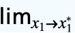
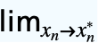
- Limit 计算函数 f 的极限值 f*,当变量 x 或 xi 任意接近它们的极限点 x* 或
 .
- 通过使用字符 ,输入为
 lim
 或 \[Limit],带有下标或上标,极限可以输入如下:
-
 f
不同方向的极限  f
上限  f
下限  f
复平面的极限  …
 f
Limit[f,{x1  ,…,xn
 }]
- 对于有限极限点 x* 和 {
 ,…,
 },有限极限值 f*:
-
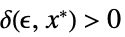
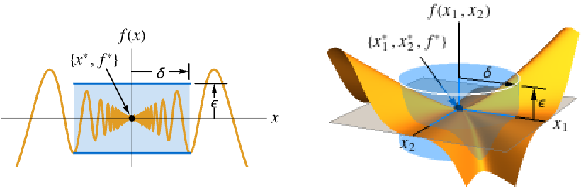
Limit[f,xx*]f* 对于每个  ,有
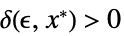 使得
 蕴涵
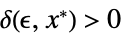
Limit[f,{x1,…,xn}{  ,…,
 }]f*
对于每个  ,有
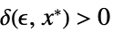 使得
 蕴涵

- 对于无穷极限点和有限极限值 f*:
-
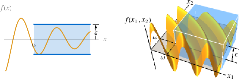
Limit[f,x∞]f* 对于每个  ,有
 使得
 蕴涵
Limit[f,{x1,…,xn}{∞,…,∞}]f* 对于每个  ,有
 使得
 蕴涵

- 当证明极限不存在时,Limit 返回 Indeterminate. 当极限不存在时,MinLimit 和 MaxLimit 可以经常被用于计算函数的最小和最大极限.
- 当没有找到极限时,Limit 返回未计算或一个 Interval. 如果返回 Interval,不保证有最小的可能区间.
- 可以给出以下选项:
-
Assumptions $Assumptions 参数上的假设 Direction Reals 接近极限点的方向 GenerateConditions Automatic 是否产生参数上的条件 Method Automatic 使用的方向 PerformanceGoal "Quality" 性能方面的优化 - Direction 的可能设置包括:
-
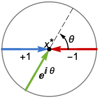
Reals 或 "TwoSided" 来自两个实方向 "FromAbove" 或 -1 来自上限或更大的值 "FromBelow" 或 +1 来自下限或更小的值 Complexes 来自所有复方向 Exp[ θ] 在方向 
{dir1,…,dirn} 对变量 xi 分别使用方向 diri - 在 x* 的 DirectionExp[ θ] 表明接近极限点 x* 的曲线的方向正切.
- GenerateConditions 的可能设置包括:
-
Automatic 只是非一般的条件 True 所有条件 False 无条件 None 如果需要条件,返回未计算的 - PerformanceGoal 的可能设置包括 $PerformanceGoal、"Quality" 和 "Speed". 当设置为 "Quality" 时,Limit 通常可以解出更多的问题或者产生更简单的结果,但是可能会耗费更多的时间和内存.
范例
打开所有单元 关闭所有单元基本范例 (3)
Limit[Sin[x] / x, x -> 0]Plot[Sin[x] / x, {x, -1, 1}, Epilog -> {PointSize[Large], Point[{0, 1}]}]Limit[(1 + Sinh[x]/Exp[x]), x -> ∞]Plot[{(1 + Sinh[x]/Exp[x]), (1/2)}, {x, 0, 10}, PlotStyle -> {Automatic, Dashed}, PlotRange -> {0, 1}]Limit[RealAbs[x] / x, x -> 0, Direction -> "FromAbove"]Limit[RealAbs[x] / x, x -> 0, Direction -> "FromBelow"]Limit[RealAbs[x] / x, x -> 0]Plot[RealAbs[x] / x, {x, -1, 1}]范围 (35)
基本用途 (5)
Limit[Sin[x], x -> π / 2]Limit[x / (x - 2a), x -> a]求在 -Infinity 的极限:
Limit[3x ^ 2 / (x ^ 2 - 2), x -> -∞]

Limit[RealAbs[x] Tan[y] ^ 2, {y -> Pi / 2, x -> 0}]

Limit[RealAbs[x]Tan[y] ^ 2, {x -> 0, y -> Pi / 2}]
Limit[(Tan[x y]/x y), {x, y} -> {0, 0}]排版极限 (4)

 输入
 创建下标:
Underscript[, x -> 0](x/x^3 + x^2) 或
 获取上下极限:
Underscript[, x -> 0^ + ](x/x^3 + x^2) 创建上标:
Underscript[, x -> 0^ - ](x/x^3 + x^2)指定 Reals 或 Complexes 的方向,在 字符上以下标形式输入域:
Underscript[, xUnderscript[ -> , ℂ]0](x/x^3 + x^2)输入规则  ->
 ,使用
 创建一个下标,然后键入
 reals
 以输入
 :
Underscript[, xUnderscript[ -> , ℝ]0](x/x^3 + x^2)TraditionalForm 格式:
Limit[f[x], x -> a, Direction -> Reals]//TraditionalForm基本函数 (6)
Limit[ a x ^ 2 + 4x + 7, x -> 1]Limit[(1/(x - 2)^2), x -> 2]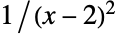

Plot[(1/(x - 2)^2), {x, 1, 3}, Epilog -> {Dashed, InfiniteLine[{2, 0}, {0, 1}]}]Limit[Sqrt[x - 1] / x, x -> 1]Limit[3(x ^ a - a x + a - 1) / (x - 1) ^ 2, x -> 1]Limit[(x - 3) / (Sqrt[x] - 3), x -> 9, Direction -> Reals]
Plot[(x - 3) / (Sqrt[x] - 3), {x, 8, 10}, ExclusionsStyle -> Dashed]Limit[Sin[2x] / Sin[x], x -> Pi]Limit[(Tan[x] - x) / x ^ 3, x -> 0]Limit[Tan[x], x -> π / 2, Direction -> -1]Plot[Tan[x], {x, 0, Pi}, ExclusionsStyle -> Dashed]Limit[Sin[1 / x], x -> 0]Plot[Sin[1 / x], {x, -.1, .1}]Limit[x^n Exp[-x^-2], x -> 0]Limit[(25 ^ x - 5 ^ x) / (4 ^ x - 2 ^ x), x -> 0]//SimplifyLimit[(1 + Sin[5x]) ^ Cot[x], x -> 0]Limit[x Log[x ^ 2], x -> 0]Limit[Log[x] / x, x -> 0]Limit[(x ^ a - 1) / a, a -> 0]Limit[Sin[x] + Log[x - a] / Log[E ^ x - E ^ a], x -> a]Limit[{Sqrt[z], Log[z]}, z -> -1, Direction -> ℝ]Limit[{Sqrt[z], Log[z]}, z -> -1, Direction -> -I]Limit[{Sqrt[z], Log[z]}, z -> -1, Direction -> I]TableForm[Table[{-1 + Δ, Sqrt[-1 + Δ], Log[-1 + Δ]}, {Δ, {0.01, -0.01, 0.01I, -0.01I}}], TableHeadings -> {None, {z, Sqrt[z], Log[z]}}]Limit[{Sqrt[z], Log[z]}, z -> -1, Direction -> ℂ]无穷处的基础函数 (4)
在 ±Infinity 处的代数函数极限:
Limit[1 / x, x -> ∞]Limit[Sqrt[x ^ 2 + a x] - Sqrt[x ^ 2 + b x], x -> ∞]Limit[a x ^ 2 / (b x ^ 2 - x), x -> -∞]在 ±Infinity 处,三角函数的极限:
Limit[Sin[x], x -> ∞]Limit[ArcTan[x ^ 3 - x], x -> -∞]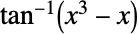
Plot[{ArcTan[x ^ 3 - x], -Pi / 2, Pi / 2}, {x, -5, 5}, PlotTheme -> "DashedLines"]Limit[x ^ 2 + x Sin[x ^ 2], x -> ∞]
Plot[x ^ 2 + x Sin[x ^ 2], {x, 0, 10}]Limit[Exp[x](Exp[1 / x - Exp[-x]] - Exp[1 / x]), x -> ∞]Plot[{Exp[x](Exp[1 / x - Exp[-x]] - Exp[1 / x]), -1}, {x, 1, 20}, PlotRange -> All, PlotTheme -> "DashedLines"]Limit[x ^ (1 / x), x -> ∞]Plot[{x ^ (1 / x), 1}, {x, 0, 40}, PlotRange -> All, PlotTheme -> "DashedLines"]Limit[(1 + a / x) ^ (b x), x -> ∞]Limit[Log[x] / Sqrt[x], x -> -∞]Limit[Exp[Exp[-x / (1 + Exp[-x])]]Exp[-x / (1 + Exp[-x] / (1 + Exp[-x]))]Exp[Exp[-x + Exp[-x / (1 + Exp[-x])]]] / (Exp[-x / (1 + Exp[-x])])^2 - Exp[x] + x, x -> ∞]Limit[(Log[Log[x] + Log[Log[x]]] - Log[Log[x]]) / Log[Log[x] + Log[Log[Log[x]]]]Log[x], x -> ∞]Limit[Exp[Log[Log[x + Exp[Log[x]Log[Log[x]]]]] / Log[Log[Log[Exp[x] + x + Log[x]]]]], x -> ∞]分段函数 (5)
f[x_] := Piecewise[{{1, x == 1}}, (x - 1) / (x ^ 2 - 1)]Limit[f[x], x -> 1, Direction -> Reals]f[1]The value of the function at  lies away from the nearby values of the function as
 :
Plot[f[x], {x, 0, 2}, Epilog -> {PointSize[Medium], RGBColor[0.24, 0.6, 0.8], Point[{1, f[1]}]}]g[x_] := Piecewise[{{1 - x ^ 2, x ≤ 0}}, x ^ 2]Limit[g[x], x -> 0, Direction -> "FromAbove"]Limit[g[x], x -> 0, Direction -> "FromBelow"]g[0]

Plot[g[x], {x, -1, 1}, Epilog -> {PointSize[Large], RGBColor[0.24, 0.6, 0.8], Point[{0, g[0]}]}]UnitStep 是高效的右连续分段函数:
Limit[UnitStep[x], x -> 0, Direction -> "FromBelow"]Limit[UnitStep[x], x -> 0, Direction -> "FromAbove"]UnitStep[0]

Plot[UnitStep[x], {x, -1, 1}, Epilog -> {RGBColor[0.24, 0.6, 0.8], PointSize[Large], Point[{0, UnitStep[0]}]}]RealSign 是高效的不连续分段函数:
Limit[RealSign[x], x -> 0, Direction -> "FromBelow"]Limit[RealSign[x], x -> 0, Direction -> "FromAbove"]RealSign[0]

Plot[RealSign[x], {x, -1, 1}, Epilog -> {RGBColor[0.24, 0.6, 0.8], PointSize[Large], Point[{0, RealSign[0]}]}]求当 x 从更大的数趋近时,Floor 的极限:
Limit[Floor[x], x -> n, Assumptions -> n∈Integers, Direction -> "FromAbove"]求当 x 从更小的数趋近时,Floor 的极限:
Limit[Floor[x], x -> n, Assumptions -> n∈Integers, Direction -> "FromBelow"]Plot[Floor[x], {x, -4, 4}, ExclusionsStyle -> Dashed]特殊函数 (4)
包含 Gamma 的极限:
Limit[Gamma[z], z -> -1, Direction -> "FromAbove"]Limit[Gamma[x + 1] ^ (1 / x) / x, x -> ∞]Plot[{Gamma[x + 1] ^ (1 / x) / x, 1 / E}, {x, 0, 30}, PlotRange -> {0, 1.2}, PlotStyle -> {Automatic, Dashed}]Limit[Gamma[x + 1 / 2] / Gamma[x] / Sqrt[x], x -> ∞]Plot[{Gamma[x + 1 / 2] / Gamma[x] / x, 1 / Sqrt[x]}, {x, 0, 10}, PlotRange -> {0, 1.2}, PlotStyle -> {Automatic, Dashed}]Limit[BesselI[1, 3x] / (x BesselI[1, x] ^ 3), x -> ∞]Plot[{BesselI[1, 3x] / (x BesselI[1, x] ^ 3), (2 π/Sqrt[3])}, {x, 0, 10}, PlotRange -> {0, 20}, PlotStyle -> {Automatic, Dashed}]Limit[x^3 HankelH1[3, x], x -> 0]Limit[x SphericalBesselJ[1, 3x], x -> ∞]Plot[x SphericalBesselJ[1, 3x], {x, 0, 10}, PlotRange -> 0.5]Limit[FresnelS[x] / x ^ 3, x -> 0]Limit[Erfc[x], x -> -∞]Plot[{Erfc[x], 2}, {x, -5, 5}, PlotStyle -> {Automatic, Dashed}]Limit[CosIntegral[x] / Log[x ^ a], x -> 0, Assumptions -> a > 0]在每个非正偶整数,Gamma 从左边趋近  ,从右边趋近
 :
Limit[Gamma[z], z -> a, Direction -> "FromAbove", Assumptions -> a∈ℤ && a ≤ 0 && Mod[a, 2] == 0]Limit[Gamma[z], z -> a, Direction -> "FromBelow", Assumptions -> a∈ℤ && a ≤ 0 && Mod[a, 2] == 0]Limit[Gamma[z], z -> a, Direction -> "FromAbove", Assumptions -> a∈ℤ && a ≤ 0 && Mod[a, 2] == 1]Limit[Gamma[z], z -> a, Direction -> "FromBelow", Assumptions -> a∈ℤ && a ≤ 0 && Mod[a, 2] == 1]嵌套的极限 (3)


Limit[ArcTan[y / x], {y -> ∞, x -> ∞}]通过计算两个 Limit 表达式,获取同样的结果:
Limit[ArcTan[Abs[y / x], x -> ∞], y -> ∞]

Limit[ArcTan[y / x], {x -> ∞, y -> ∞}]Limit[Limit[ArcTan[y / x], y -> ∞], x -> ∞]


Limit[Exp[(y x^2/Sqrt[x^3 + y^2x^4 ])], {y -> -∞, x -> 0}]


Limit[Exp[(y x^2/Sqrt[x^3 + y^2x^4 ])], {x -> 0, y -> -∞}]f[x_, y_] := (y /x + y )


Limit[f[x, y], {y -> 0, x -> 0}]


Limit[f[x, y], {x -> 0, y -> 0}]Limit[f[x, y], {x, y} -> {0, 0}]Show[Plot3D[f[x, y], {x, y}∈Disk[{0, 0}, 2], ClippingStyle -> None, Mesh -> None, BoxRatios -> 1], ParametricPlot3D[{{t, 0, f[t, 0]}, None, {0, t, f[0, t]}}, {t, -2, 2}, PlotStyle -> Thickness[0.025], PlotLegends -> LineLegend[{y == 0, None, x == 0}]], ViewPoint -> {-3, 1, 1}]多变量极限 (4)

f[x_, y_] := (3 x^2 y - 3 x^2/1 + x^2 - 2 y + y^2)




Limit[f[x, 0], {x, y} -> {0, 1}]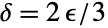
Reduce[(0 < Sqrt[x ^ 2 + (y - 1) ^ 2] < 2ϵ / 3)(Abs[f[x, y] - 0] < ϵ), a, Reals]
Plot3D[{f[x, y], (3/2)Sqrt[x ^ 2 + (y - 1) ^ 2], (-3/2)Sqrt[x ^ 2 + (y - 1) ^ 2]}, {x, y}∈Disk[{0, 1}, 1], BoxRatios -> 1, PlotStyle -> {Automatic, Opacity[.75], Opacity[.75]}]f[x_, y_] := ArcTan[y ^ 2 / (x ^ 2 + x ^ 3)]Limit[f[x, y], {x -> 0, y -> 0}]Limit[f[x, y], {y -> 0, x -> 0}]
Limit[f[x, x], x -> 0]Limit[f[x, -x], x -> 0]Limit[f[x, y], {x, y} -> {0, 0}]Plot3D[f[x, y], {x, -1, 1}, {y, -1, 1}, ViewPoint -> {-1, -.5, 1.5}]f[x_, y_] := (x ^ 3 + y ^ 3) / (x ^ 2 + y ^ 2)Limit[f[x, y], {x, y} -> {0, 0}]{x[r_, θ_], y[r_, θ_]} := {r Cos[θ], r Sin[θ]};Simplify[f[x[r, θ], y[r, θ]]]
Limit[f[x[r, θ], y[r, θ]], r -> 0, Direction -> -1]ParametricPlot3D[{x[r, θ], y[r, θ], f[x[r, θ], y[r, θ]]}, {r, 0, 3}, {θ, 0, 2Pi}, ViewPoint -> {-1.5, -2, 1.5}]f[x_, y_, z_] := (x z/x^2 + y^2 + z^2)Limit[f[x, y, z], {x, y, z} -> {0, 0, 0}]

{Limit[f[x, y, 0], {x, y} -> {0, 0}], Limit[f[0, y, z], {y, z} -> {0, 0}]}
Limit[f[x, 0, z], {x, z} -> {0, 0}]SliceContourPlot3D[f[x, y, z], {x, y, z}∈Ball[]]选项 (13)
Assumptions (2)
使用 Assumptions 指定参数上的条件:
Limit[x ^ a, x -> ∞, Assumptions -> a < 0]Limit[x ^ a, x -> ∞, Assumptions -> a == 0]Limit[x ^ a, x -> ∞, Assumptions -> a > 0]Limit[a ^ x / x ^ a, x -> ∞, Assumptions -> a > 1]Limit[a ^ x / x ^ a, x -> ∞, Assumptions -> 0 < a < 1]Direction (5)
Limit[1 / x, x -> 0, Direction -> "FromBelow"]Limit[1 / x, x -> 0, Direction -> 1]Limit[1 / x, x -> 0, Direction -> "FromAbove"]Limit[1 / x, x -> 0, Direction -> -1]Limit[FractionalPart[x ^ 2]Sin[x], x -> 2, Direction -> "FromBelow"]Limit[FractionalPart[x ^ 2]Sin[x], x -> 2, Direction -> "FromAbove"]Limit[FractionalPart[x ^ 2]Sin[x], x -> 2, Direction -> "TwoSided"]Plot[FractionalPart[x ^ 2]Sin[x], {x, 0, 7}]Limit[Tan[x], x -> π / 2, Direction -> "FromBelow"]Limit[Tan[x], x -> π / 2, Direction -> "FromAbove"]Limit[Tan[x], x -> π / 2, Direction -> ℝ]Limit[Tan[x], x -> π / 2, Direction -> ℂ]Limit[EllipticK[2 + x], x -> 0, Direction -> +I]Limit[EllipticK[2 + x], x -> 0, Direction -> Reals]Limit[EllipticK[2 + x], x -> 0, Direction -> -I]Limit[EllipticK[2 + x], x -> 0, Direction -> Complexes]f[x_, y_] := (x y/x + y)(2 + RealSign[ x y] + RealSign[y])Limit[f[x, y], {x, y} -> {0, 0}, Direction -> "FromAbove"]Limit[f[x, y], {x, y} -> {0, 0}, Direction -> {"FromAbove", "FromAbove"}]Limit[f[x, y], {x, y} -> {0, 0}, Direction -> {"FromBelow", "FromAbove"}]Limit[f[x, y], {x, y} -> {0, 0}, Direction -> {"FromBelow", Reals}]Limit[f[x, y], {x, y} -> {0, 0}, Direction -> {Reals, "FromBelow"}]Row@{Plot3D[f[x, y], {x, y}∈Disk[], Exclusions -> {{x == -y , x <= 0}}, ClippingStyle -> None, ImageSize -> 200], DensityPlot[f[x, y], {x, -1, 1}, {y, -1, 1}, Exclusions -> {{x == -y , x <= 0}}, ClippingStyle -> Automatic, ImageSize -> Small]}GenerateConditions (3)
Limit[x ^ n, x -> 0, GenerateConditions -> False]Limit[x ^ n, x -> 0]Limit[Exp[a x], x -> ∞, GenerateConditions -> None]Limit[Exp[a x], x -> ∞]Limit[(x y/(x - a)^2 + y^2), {x, y} -> {0, 0}]当 GenerateConditions->True,甚至会报告这些非通用条件:
Limit[(x y/(x - a)^2 + y^2), {x, y} -> {0, 0}, GenerateConditions -> True]Method (2)
使用 Method{"AllowIndeterminateOutput"False} 避免 Indeterminate 结果:
Limit[1 / x, x -> 0]Limit[1 / x, x -> 0, Method -> "AllowIndeterminateOutput" -> False]
Plot[1 / x, {x, -1, 1}]对于振荡函数,边界会作为 Interval 对象返回:
Limit[Sin[x], x -> ∞, Method -> {"AllowIndeterminateOutput" -> False}]Limit[Cos[π / x] / x, x -> 0, Method -> "AllowIndeterminateOutput" -> False]{Plot[Sin[π x], {x, 0, 10.5}], Plot[Cos[π / x] / x, {x, -0.25, 0.25}, PlotRange -> 50]}使用 Method{"AllowIntervalOutput"False} 避免 Interval 对象结果:
Limit[Sin[Pi / x], x -> 0, Method -> "AllowIndeterminateOutput" -> False]Limit[Sin[Pi / x], x -> 0, Method -> {"AllowIndeterminateOutput" -> False, "AllowIntervalOutput" -> False}]
Plot[Sin[π / x], {x, -0.25, 0.25}]PerformanceGoal (1)
使用 PerformanceGoal 避免潜在的昂贵计算:
expr = (2 y z^2 - z^3 + y (x - 2 y + 3 z)^2 - z (x - 2 y + 3 z)^2/y^2 - 2 y z + z^2 - y (x - 2 y + 3 z) + z (x - 2 y + 3 z) + (x - 2 y + 3 z)^2);Limit[expr, {x, y, z} -> {0, 0, 0}, PerformanceGoal -> "Speed"]Limit[expr, {x, y, z} -> {0, 0, 0}]应用 (23)
极限几何 (5)


f[x_] := (Cos[x] - Exp[x]/x )Limit[f[x], x -> 0, Direction -> Reals]


NumberForm[TableForm[Table[{x, f[x]}, {x, {.1, .05, 0.01, .005, 0.001, 0.0001}}], TableHeadings -> {{}, {x, HoldForm@f[x]}}], {4, 4}]Plot[{f[x], -1}, {x, -1, 1}, PlotStyle -> {Automatic, Dashed}]

f[0]



f[x_] := Sin[Tan[x]]Limit[f[x], x -> Pi / 2, Direction -> Reals]
g[x_] := Cos[x]Sin[Tan[x]]Limit[g[x], x -> Pi / 2, Direction -> Reals]在增加的  周围的小区域,
 连续在
 之间弹跳,但是
 在平坦的增加:
Manipulate[Plot[{f[x], g[x]}, {x, Pi / 2 - a, Pi / 2 + a}], {a, 1, 0.001}, SaveDefinitions -> True]
r[x_] := (x^4 - 6 x^3 + 11 x^2 - 6 x/x - 1)Limit[r[x], x -> 1]

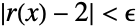
Reduce[ForAll[x, 0 < RealAbs[x - 1] < δ, RealAbs[r[x] - 2] < ϵ], δ, Reals]
Simplify[%, 0 < ϵ < 2] 的图总是通过边,不是顶部或底部“离开”中心在
 ,高为
 ,宽为
 的长方形:
With[{δ = Root[ϵ - #1 - 2 #1^2 + #1^3&, 2]}, Manipulate[Plot[r[x], {x, -1, 3}, PlotRange -> {-2, 4}, Epilog -> {AbsolutePointSize[Large], Point[{1, 2}], FaceForm[Directive[StandardBlue, Opacity[0.5]]], Rectangle[{1 - δ, 2 - ϵ}, {1 + δ, 2 + ϵ}]}, PlotLabel -> StringForm["ϵ=`1`, δ=`2`", ToBoxes[ϵ], ToBoxes[δ]]], {ϵ, 2, 0}, SaveDefinitions -> True]]f[x_] := (x ^ 2 + 1) / (x - 2x ^ 2 + 3)sol = Solve[Denominator[f[x]] == 0, x]
{Limit[f[x], x -> -1, Direction -> "FromAbove"], Limit[f[x], x -> -1, Direction -> "FromBelow"]}{Limit[f[x], x -> (3/2), Direction -> "FromAbove"], Limit[f[x], x -> (3/2), Direction -> "FromBelow"]}
{Limit[f[x], x -> ∞], Limit[f[x], x -> -∞]}Plot[{f[x], -1 / 2}, {x, -3, 3}, PlotStyle -> {Automatic, Dashed}, ExclusionsStyle -> Dashed, PlotRange -> 5]f[x_] := (x ^ 2 + 3) / (2 x + 1)m = Limit[f[x] / x, x -> ∞]b = Limit[f[x] - m x, x -> ∞]Plot[{f[x], m x + b}, {x, 0, 10}, PlotStyle -> {Automatic, Dashed}]不连续性 (5)
f[x_] := (3^1 / x - 3^-1 / x/3^1 / x + 3^-1 / x)FunctionDomain[f[x], x]Limit[f[x], x -> 0]Limit[f[x], x -> 0, Direction -> "FromBelow"]Limit[f[x], x -> 0, Direction -> "FromAbove"]Plot[f[x], {x, -3, 3}]f[x_] := Piecewise[{{Sin[2*x]/(1 - Exp[-2*x]), x > 0}, {2, x == 0}, {(1 - Cos[x]^2)/x^2, x < 0}}]f[0]Limit[f[x], x -> 0]f[x_] := Piecewise[{{1, x == 1}, {3, x == 3}}, x ^ -2]FunctionDomain[f[x], x]函数两边趋向于 Infinity,因此它是无穷不连续:
Limit[f[x], x -> 0]Solve[Limit[f[x], x -> a] ≠ f[a], a]Limit[f[x], x -> 3]

f[x_] := Sin[3x] / Tan[2x]
f[0]



Simplify[Limit[f[x], x -> n Pi, Assumptions -> n∈Integers], Mod[n, 2] == 0]
Simplify[Limit[f[x], x -> n Pi, Assumptions -> n∈Integers], Mod[n, 2] == 1]
Limit[f[x], x -> n Pi + (Pi/2), Assumptions -> n∈Integers ]


g[x_] := Piecewise[{{3/2, Mod[x, 2*Pi] == 0}, {-3/2, Mod[x, 2*Pi] == Pi}, {f[x], True}}]
g[0] == Limit[g[x], x -> 0]

Plot[{g[x], f[x]}, {x, -2Pi, 2Pi}, ExclusionsStyle -> Dotted]f[x_, y_] := UnitStep[x]Sin[2y] / xLimit[f[x, y], {x, y} -> {0, 0}]左半平面存在极限是 0,因此任何从那里趋近的射线有同样的极限:
Limit[f[x, y], {x, y} -> {0, 0}, Direction -> {"FromBelow", Reals}]

Limit[f[x, y] /. Thread[{x, y} -> {0, 0} + {1, m}t], t -> 0, Direction -> "FromAbove"]
Show[Plot3D[f[x, y], {x, -Pi, Pi}, {y, -Pi, Pi}, Mesh -> None, ClippingStyle -> None, PlotRange -> 2], ParametricPlot3D[{{-t, -t, f[-t, -t]}, {-t, t, f[-t, t]}, {t, t, f[t, t]}, {t, -t, f[t, -t]}}, {t, 0, Pi}, PlotStyle -> Thickness[0.025], PlotLegends -> LineLegend[{x == y && x < 0, x == -y && x < 0, x == y && x > 0, x == -y && x > 0}]], ViewPoint -> {.7, -1.8, 2.8}]导数 (5)

f[x_] := Sin[x]Exp[x]DifferenceQuotient[f[x], {x, h}]
Limit[%, h -> 0]

f[x_] := Piecewise[{{x^2 + 2*x - 1, x >= 0}, {x^3 - 1, True}}]
Limit[(f[0 + h] - f[0]/h), h -> 0]{Underscript[, h -> 0^ + ](f[0 + h] - f[0]/h), Underscript[, h -> 0^ - ](f[0 + h] - f[0]/h)}
{Underscript[, x -> 0^ + ]f'[x], Underscript[, x -> 0^ - ]f'[x]}可视化  和其导数;前者在 0 处有“扭结”,后者是跳跃不连续:
Plot[{f[x], f'[x]}, {x, -1, 1}, ExclusionsStyle -> Dashed, AxesOrigin -> {-1, 0}]

f[x_] := Piecewise[{{0, x == 0}, {x^2*Sin[1/x], True}}]
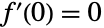
Subscript[p, x] = Limit[(f[1 + h, 2] - f[1, 2]/h), h -> 0]


Limit[f'[x], x -> 0]

f[x_, y_] := Piecewise[{{0, x == 1 && y == 2}, {(-6 + 8*x - 2*x^2 + 5*y - 6*x*y + x^2*y - y^2 + x*y^2)/
(5 - 2*x + x^2 - 4*y + y^2), True}}]Subscript[p, x] = Limit[(f[1 + h, 2] - f[1, 2]/h), h -> 0]Subscript[p, y] = Limit[(f[1, 2 + h] - f[1, 2]/h), h -> 0]

Limit[(RealAbs[f[x, y] - f[1, 2] - {Subscript[p, x], Subscript[p, y]}.({x, y} - {1, 2})]/Norm[{x, y} - {1, 2}]), {x, y} -> {1, 2}]Plot3D[f[x, y], {x, 0, 2}, {y, 1, 3}]
Grad[f[x, y], {x, y}]//Simplify
Limit[%, {x, y} -> {1, 2}]f[x_, y_] = Exp[a x]Cos[b y]Limit[DifferenceQuotient[f[x, y], {x, h}], h -> 0] == D[f[x, y], x]Limit[DifferenceQuotient[f[x, y], {x, 2, h}], h -> 0] == D[f[x, y], {x, 2}]
Limit[DifferenceQuotient[f[x, y], {x, 2, h}, {y, 3, k}], {h, k} -> {0, 0}]% == D[f[x, y], {x, 2}, {y, 3}]数学常数和表达式 (4)
计算出  是 Infinity 处的极限:
Limit[(1 + 1 / x) ^ x, x -> ∞]Limit[(1 + x) ^ (1 / x), x -> 0]计算出  是 Gamma 函数的极限:
Limit[(2 ^ (4 x + 1) Gamma[x + 1] ^ 4) / ((2 x + 1) Gamma[2x + 1] ^ 2), x -> ∞]计算出 EulerGamma 是涉及 Zeta 函数的极限:
Limit[Zeta[x] - 1 / (x - 1), x -> 1]计算出 EulerGamma 是指数积分的极限:
Limit[ExpIntegralEi[Log[1 + x]] + Log[1 - 1 / x] - ExpIntegralEi[Log[x]] - I Pi, x -> 0, Direction -> -1]其他应用 (4)
如果 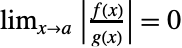 ,函数
 在
 处是 "little-o of
 ",写作
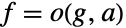 :
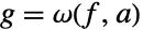
o[x_, a_][f_, g_] := Replace[Underscript[, xUnderscript[ -> , ℝ]a]Abs[(f/g)] == 0, Indeterminate == _ -> False]类似,如果  ,
 是 "little-omega of
 ",写作
 :
ω[x_, a_][f_, g_] := Replace[Underscript[, xUnderscript[ -> , ℝ]a]Abs[(f/g)] == ∞, Indeterminate == _ -> False]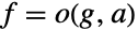
{o[x, 0][x^3, 10x^2 + 5x + 1], ω[x, 0][10x^2 + 5x + 1, x^3]}{o[x, 0][1, Cos[x]], ω[x, 0][1, Cos[x]]}{o[x, a][f[x], f[x]], ω[x, 0][f[x], f[x]]}

funs = {x ^ 2, 1, x, x Log[x], Cos[x]};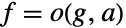


Sort[funs, o[x, 0]]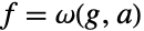
Sort[funs, ω[x, 0]]

% === Reverse[%%]



f[x_] := Exp[x]
t[n_, a_][x_] := Sum[(D[f[x], {x, k}] / k! /. x -> a)(x - a)^k, {k, 0, n}]
t[5, 1][x]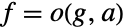
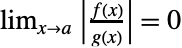
o[x_, a_][f_, g_] := Replace[Underscript[, xUnderscript[ -> , ℝ]a]Abs[(f/g)] == 0, Indeterminate == _ -> False]
o[x, 1][f[x] - t[5, 1][x], (x - 1)^5]

keRelativistc[v_] := (m Quantity[1, "SpeedOfLight"]^2/Sqrt[1 - v^2 / Quantity[1, "SpeedOfLight"]^2]) - m Quantity[1, "SpeedOfLight"]^2keClassical[v_] := (1/2)m v^2Limit[(keRelativistc[v]/keClassical[v]), v -> 0]Integrate[1 / x ^ 2, {x, 1, a}, Assumptions -> a > 0]Limit[%, a -> ∞]Integrate[1 / x ^ 2, {x, 1, ∞}]属性和关系 (14)
f[x_] := x ^ 3Limit[c f[x], x -> a] == c Limit[f[x], x -> a]如果 f 和 g 具有有限极限,它们的和的 Limit 是可分配的:
f[x_] := x ^ 2g[x_] := 5x - 3Limit[f[x] + g[x], x -> a] == Limit[f[x], x -> a] + Limit[g[x], x -> a]如果 f 和 g 具有有限极限,它们的积的 Limit 是可分配的:
f[x_] := 5xg[x_] := 5 - x ^ 2Limit[f[x] g[x], x -> a] == Limit[f[x], x -> a] Limit[g[x], x -> a]f[x_] := (1 + 1 / x) ^ xLimit[f[x] ^ m, x -> ∞] == Limit[f[x], x -> ∞] ^ mf[x_] := Sin[x]g[x_] := (x + 1) / x;Limit[f[g[x]], x -> 1] == f[Limit[g[x], x -> 1]]h[n_] := Ceiling[n]Limit[h[g[x]], x -> 1] === h[Limit[g[x], x -> 1]]Limit[x Sin[1 / x], x -> 0]
Reduce[-RealAbs[x] ≤ x Sin[1 / x] ≤ RealAbs[x]]//SimplifyLimit[Abs[x], x -> 0]Plot[{x Sin[1 / x], RealAbs[x], -RealAbs[x]}, {x, -1, 1}, Filling -> {2 -> {3}}]Limit[Sin[x] / x, x -> ∞]
Reduce[(-1/x) ≤ (Sin[x]/x) ≤ (1/x)]Limit[1 / x, x -> ∞]Plot[{Sin[x] / x, 1 / x, -1 / x}, {x, 0, 50}, PlotRange -> 0.35, Filling -> {2 -> {3}}]Assumptions 应用于极限表达式中的参数:
Limit[Tan[x], x -> π / 2 + n π, Direction -> -1, Assumptions -> n∈Integers]Direction 把条件放在极限变量上:
Limit[Tan[x], x -> π / 2 + n π, Direction -> 1, Assumptions -> n∈Integers]Plot[Tan[x], {x, -2π, 2π}, ExclusionsStyle -> Dashed]Limit[(f[h + x] - f[x]/h), h -> 0, Analytic -> True]f[x_] := Erf[x]g[x_] := xLimit[f[x], x -> 0] == Limit[g[x], x -> 0] == 0Limit[f[x] / g[x], x -> 0] == Limit[f'[x] / g'[x], x -> 0](f'[0]/g'[0])如果存在 Limit,那么也有 DiscreteLimit,它们有同样的值:
f[n_] := n / (n + 1)Limit[f[n], n -> ∞]DiscreteLimit[f[n], n -> ∞]g[n_] := Sin[n π]DiscreteLimit[g[n], n -> ∞]Limit[g[n], n -> ∞]Show[Plot[g[n], {n, 0, 10}], DiscretePlot[g[n], {n, 0, 10}, PlotMarkers -> {"Point", Medium}]]如果存在 Limit,那么 MaxLimit 也是,它有同样的值:
f[x_] := Sin[x] / xLimit[f[x], x -> ∞]MaxLimit[f[x], x -> ∞]如果存在 Limit,那么 MinLimit 也是,它有同样的值:
f[x_] := Sin[x] / xLimit[f[x], x -> ∞]MinLimit[f[x], x -> ∞]f = Sin[2 ^ x] ^ 2 + x / 3;Limit[f, x -> 1] == (f /. x -> 1)用 FunctionContinuous 测试函数是否是连续的:
FunctionContinuous[f, x]可能存在的问题 (1)
对于非精确输入,Limit 可能返回一个不准确的答案:
Limit[Log[1 - (Log[Exp[z] / z - 1] + Log[z]) / z] / z, z -> 100.]Limit[Log[1 - (Log[Exp[z] / z - 1] + Log[z]) / z] / z, z -> 100]{N[%], N[%, 20]}互动范例 (1)
Manipulate[
	Graphics[{EdgeForm[Opacity[1]], {StandardGray, Disk[{0, 0}, 1, {0, θ}], LightDarkSwitched@White, Polygon[{{0, 0}, {Cos[θ], Sin[θ]}, {Cos[θ], 0}}], AbsoluteDashing[{5, 2}], Line[{{Cos[θ], Sin[θ]}, {0, 0}, {Cos[θ], 0}}], StandardBlue, Polygon[{{1, 0}, {Cos[θ], Sin[θ]}, {Cos[θ], 0}}]}, Style[{Text[ϕ, .1{Cos[θ / 2], Sin[θ / 2]}]}, 15]}, PlotRange -> {{-.1, 1.2}, {-.3, 1.1}}, ImageSize -> {400, 300}, AspectRatio -> Automatic,
	PlotLabel -> Style[HoldForm@(t[ϕ]/s[ϕ]) == NumberForm[((-1 + Cos[θ]) Sin[θ]/-θ + Cos[θ] Sin[θ]), {7, 6}], 18]
	],
Row[{Control[{{θ, π / 4.}, π / 2, .001, Slider}], " ", Dynamic[Floor[180 θ / π]], "°"}]]t[ϕ_] := (1/2)r^2(1 - Cos[ϕ]) Sin[ϕ]s[ϕ_] := (1/2)r^2(ϕ - Cos[ϕ]Sin[ϕ])Limit[t[ϕ] / s[ϕ], ϕ -> 0]巧妙范例 (2)
Limit[With[{n = 5}, 1 / 2 (2n + 1)!! / h ^ (n + 1) Integrate[LegendreP[n, t / h] f[x + t], {t, -h, h}]], h -> 0, Analytic -> True]f[x_] := {1 / x ^ 2, Sin[8x] / (6x), 3x ^ 4 / (x ^ 4 + 4), E ^ x, Sin[30 / x], x ^ 2Cos[4x ^ 2] / (x ^ 2 + 1)}a = {0, ∞, ∞, ∞, 0, ∞};range = {{0, 5}, {-0.5, 1.5}, {-2, 4}, {0, 25}, {-2, 2}, {-2, 2}};asym = {6Sign[x + 0.05], 0.02, 3, 0, {-1, 1}, {-1, 1}};Grid[Partition[Table[With[{r1 = f[x][[n]], r2 = a[[n]], r3 = range[[n]], r4 = asym[[n]]},
Plot[{r1, r4}, {x, -4, 4}, PlotRange -> r3, ImageSize -> 210, PlotStyle -> {Automatic, {StandardBlue, Dashed}, {StandardBlue, Dashed}}, ExclusionsStyle -> {{StandardBlue, AbsoluteThickness[3], Dashed}}, PlotLabel -> Style[HoldForm[Limit[r1, x -> r2]] == Limit[f[x][[n]], x -> r2], ScriptLevel -> 0]]], {n, 1, 6}], 2], Frame -> All]文本
Wolfram Research (1988),Limit,Wolfram 语言函数,https://reference.wolfram.com/language/ref/Limit.html (更新于 2017 年).
CMS
Wolfram 语言. 1988. "Limit." Wolfram 语言与系统参考资料中心. Wolfram Research. 最新版本 2017. https://reference.wolfram.com/language/ref/Limit.html.
APA
Wolfram 语言. (1988). Limit. Wolfram 语言与系统参考资料中心. 追溯自 https://reference.wolfram.com/language/ref/Limit.html 年