



StateFeedbackGains
StateFeedbackGains[sspec,{p1,…,pn}]
閉ループ系の極を piに置くような状態指定 sspec の状態フィードバックゲインを与える.
StateFeedbackGains[…,"prop"]
特性"prop"の値を与える.
詳細とオプション
- StateFeedbackGainsは極配置ゲインあるいは固有値の配置としても知られている.
- StateFeedbackGainsは,調整コントローラまたは追跡コントローラを計算するために使われる.
- StateFeedbackGainsは閉ループ系の極を位置 piに変更することで動作する.
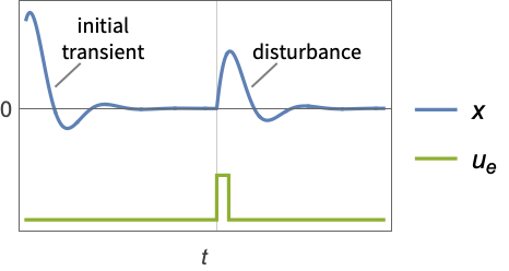
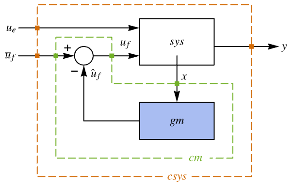
- 調整コントローラは系を押し出そうとする外乱
 にもかかわらず,系を平衡状態に保とうとする.典型的な例として,倒立振子を直立位置に保つことや航空機の水平飛行を保つこと等がある.
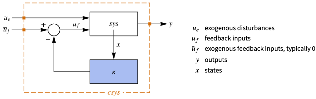
- 調整コントローラは
 の形式の制御法則で与えられる.ただし,
 は計算されたゲイン行列である.
- 置くべき極の数 n は系 sys のSystemsModelOrderで与えられる.
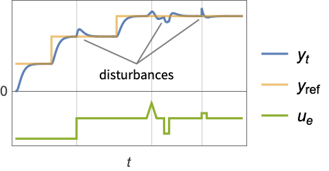
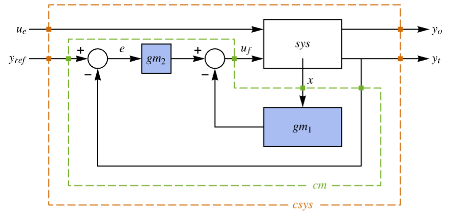
- 追跡コントローラは干渉する外乱
 があっても参照信号を追跡しようとする.典型的な例として,車のクルーズコントロールやロボットの経路追跡がある.
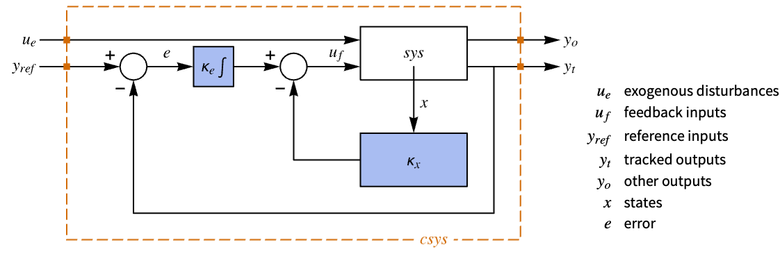
- 追跡コントローラは
 の形の制御法則によって与えられる.ただし,
 は系 sys と
 のダイナミクスを含む拡張された系の計算されたゲイン行列である.
- 置くべき極の数 n は
 で与えられる.ただし,
 は sys の SystemsModelOrderで,
 は yrefの次数で,
 は信号 yrefの数で与えられる.
- 極の配置設計はStateSpaceModelで指定されるような線形系に使うことができる.
-

連続時間系 
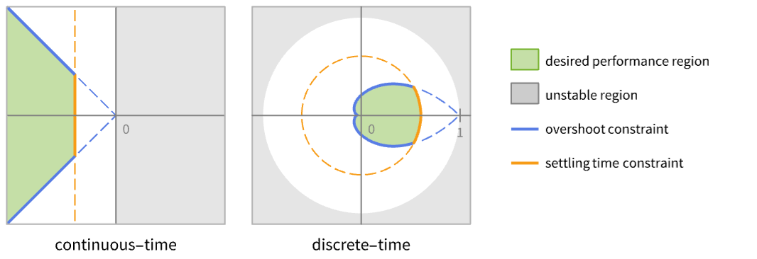
離散時間系 - 結果の閉ループ系 csys のパフォーマンスは主に極 piの位置によって決まる.
- 通常,整定時間等のパフォーマンスの制約とオーバーシュート等の品質の制約がある.これらは望ましい極位置である特定の領域に対応する.
- 系の指定 sspec は sys と uf,yt,yrefの指定である.
- 系の指定 sspec は以下の形でよい.
-
StateSpaceModel[…] 線形制御入力と線形状態 AffineStateSpaceModel[…] 線形制御入力と非線形状態 NonlinearStateSpaceModel[…] 非線形制御入力と非線形状態 SystemModel[…] 一般的な系のモデル <…> Associationとして与えられる詳細な系の指定 - 系の指定の詳細は次のキーを持つことができる.
-
"InputModel" sys モデルの任意のもの "FeedbackInputs" All フィードバック入力 uf "TrackedOutputs" None 追跡された出力 yt "TrackedSignal" Automatic yrefのダイナミクス - 追跡された信号のダイナミクスは参照信号と時間変数の関数として与えられ,デフォルトで,一定しているとみなされる.
-
Function[{r, t},r'[t]] 連続時間系 Function[{r,k},r[k+1]-r[k]] 離散時間系 - フィードバック入力と追跡された出力は次の形でよい.
-
{num1,…,numn} StateSpaceModel,AffineStateSpaceModel,NonlinearStateSpaceModelで使われる番号付きの入力 numi {name1,…,namen} SystemModelで使われる名前付きの入力 namei All すべての入力を使う - AffineStateSpaceModel,NonlinearStateSpaceModel,SystemModelのような非線形系については, 系は保存された動作点の周りで線形化される.
- StateFeedbackGains[…,"Data"]は,cd["prop"]の形で追加的な特性の抽出に使えるSystemsModelControllerDataオブジェクト cd を返す.
- StateFeedbackGains[…,"prop"]を使って cd["prop"]の値を直接得ることができる.
- 次は,特性"prop"の可能な値である.
-
"BlockDiagram" csys のブロック図 {"BlockDiagram",<"SampledData"True>} csys のサンプルデータブロック図を作成する "ClosedLoopPoles" 線形化された"ClosedLoopSystem"の極 "ClosedLoopSystem" 系 csys {"ClosedLoopSystem", cspec} 閉ループ系の形に対する詳細な制御 "ControllerModel" モデル cm "Design" コントローラ設計のタイプ "DesignModel" 設計に使われるモデル "FeedbackGains" ゲイン行列 κ またはそれに相当するもの "FeedbackGainsModel" モデル gm あるいは{gm1,gm2} "FeedbackInputs" フィードバックに使われる sys の入力 uf "InputModel" 入力モデル sys "InputCount" sys の入力 u の数 "OpenLoopPoles" "DesignModel"の極 "OutputCount" システムの出力 y の数 "SamplingPeriod" sys のサンプリング周期 "StateCount" sys の状態 x の数 "TrackedOutputs" 追跡された sys の出力 yt - 次は,cspec の可能なキーである.
-
"InputModel" csys の入力モデル "Merge" csys をマージするかどうか "ModelName" csys の名前 "SamplingPeriod" サンプルされたデータ csys を作成する - 次は,調整器のレイアウトの図である.
- 次は,追跡器のレイアウトの図である.
- StateFeedbackGainsは以下の設定のMethodオプションを取る.
-
Automatic メソッドの自動選択 "Ackermann" Ackermann法 "KNVD" Kautsky–Nichols–Van Dooren法
例題
すべて開く すべて閉じる例 (3)
フィードバック uf,外因性入力 ue での系の指定 sspec に対するフィードバックゲイン:
sspec = <|"InputModel" -> StateSpaceModel[{{{0, 1}, {1, 2}}, {{1, 0}, {1, 2}}, {{0, 1}}, {{0, 0}}}, SamplingPeriod -> None,
SystemsModelLabels -> {{uf, ue}}], "FeedbackInputs" -> 1|>;p = {-4 + 3I, -4 - 3I};StateFeedbackGains[sspec, p]nsys = NonlinearStateSpaceModel[{{-1 + Subscript[x, 2],
u + Subscript[x, 1] - 2*Subscript[x, 2]},
{Subscript[x, 1] + Subscript[x, 2]}},
{{Subscript[x, 1], 1}, {Subscript[x, 2], 1}}, {{u, 1}},
{Automatic}, Automatic, SamplingPeriod -> None];p = {-2 + I, -2 - I};StateFeedbackGains[nsys, p]StateFeedbackGains[StateSpaceModel[nsys], {-2 + I, -2 - I}]𝒸𝒹 = StateFeedbackGains[StateSpaceModel[{{{0, 5}, {-1, 2.5}}, {{0}, {1}}, {{1, 1}}, {{0}}}, SamplingPeriod -> None,
SystemsModelLabels -> None], {-2, -1.5}, "Data"]PoleZeroPlot[Table[𝒸𝒹[prop], {prop, {"InputModel", "ClosedLoopSystem"}}], IconizedObject[«plotOpts»]]スコープ (34)
基本的な用法 (8)
閉ループの極を p に置く状態フィードバックゲインを計算する:
ssm = StateSpaceModel[{{{a}}, {{b}}, {{c}}, {{d}}},
SamplingPeriod -> None, SystemsModelLabels -> None];κ = StateFeedbackGains[ssm, {p}]SystemsModelStateFeedbackConnect[ssm, κ]ssm = StateSpaceModel[{{{2}}, {{1}}, {{1}}, {{0}}}, SamplingPeriod -> None, SystemsModelLabels -> None];κ = StateFeedbackGains[ssm, {-1}]
csys = SystemsModelStateFeedbackConnect[ssm, κ]Table[Expand[OutputResponse[sys, 1, t]], {sys, {ssm, csys}}];ssm = StateSpaceModel[{{{0, 1}, {-1, -2}}, {{0}, {1}}, {{1, 0}}, {{0}}}, SamplingPeriod -> None,
SystemsModelLabels -> None];κ = StateFeedbackGains[ssm, {-2, -3}]Dimensions[κ]ssm = StateSpaceModel[{{{0, 0, -0.1}, {1., 0., -1.08}, {0., 1., -0.9}}, {{1, 1}, {1, 0}, {0, 0}},
{{0, 0, 1}}, {{0, 0}}}, SamplingPeriod -> None, SystemsModelLabels -> None];StateFeedbackGains[ssm, {-1, -2, -2.5}]//MatrixFormssm = StateSpaceModel[{{{0, 1}, {-2, -3}}, {{0}, {1}}, {{2, 0}}, {{0}}}, SamplingPeriod -> None,
SystemsModelLabels -> None];StateFeedbackGains[ssm, {-2 + I , -2 - I}]StateFeedbackGains[ssm, {-2 , -2 - I}]ssm = StateSpaceModel[{{{0, 0, -0.1}, {1., 0., -1.08}, {0., 1., -0.9}}, {{1, 1}, {1, 0}, {0, 0}},
{{0, 0, 1}}, {{0, 0}}}, SamplingPeriod -> None, SystemsModelLabels -> None];StateFeedbackGains[ssm, {-1 + I , -1 - I, -2}]極が複素共役ではないなら,コントロールは複素数で入力の一つしか使わない:
κ = StateFeedbackGains[ssm, {-1 + I , -1, -2}]Position[κ, {0..}]ssm = StateSpaceModel[{{{0, 0, -0.1}, {1., 0., -1.08}, {0., 1., -0.9}}, {{1, 1}, {1, 0}, {0, 0}},
{{0, 0, 1}}, {{0, 0}}}, SamplingPeriod -> None, SystemsModelLabels -> None];
p = {-1 + I , -1 - I, -2};StateFeedbackGains[<|"InputModel" -> ssm, "FeedbackInputs" -> {1}|>, p]StateFeedbackGains[<|"InputModel" -> ssm, "FeedbackInputs" -> {2}|>, p]StateFeedbackGains[<|"InputModel" -> ssm, "FeedbackInputs" -> {1, 2}|>, p]assm = AffineStateSpaceModel[{{E^(1 - Subscript[x, 1]) + Subscript[x, 2],
Subscript[x, 1] - Subscript[x, 2]},
{{Subscript[x, 1]}, {0}}, {Subscript[x, 1]}, {{0}}},
{{Subscript[x, 1], 1}, {Subscript[x, 2], 1}}, {{u, -2}},
{Automatic}, Automatic, SamplingPeriod -> None]StateFeedbackGains[assm, {-2, -3}]StateFeedbackGains[StateSpaceModel[assm], {-2, -3}]工場モデル (6)
連続時間StateSpaceModel:
StateFeedbackGains[StateSpaceModel[{{{0, 1.}, {-1, -1.6}}, {{0}, {1}}, {{1, 1}}, {{0}}}, SamplingPeriod -> None,
SystemsModelLabels -> None], {-1.5 + I, -1.5 - I}]離散時間StateSpaceModel:
StateFeedbackGains[StateSpaceModel[{{{0, 1.}, {0.020000000000000004, 0.1}}, {{0}, {1}}, {{1, 0}}, {{0}}},
SamplingPeriod -> τ, SystemsModelLabels -> None], {0, 0.1}]ディスクリプタStateSpaceModel:
StateFeedbackGains[StateSpaceModel[{{{-6, -4}, {-6, -5}}, {{1}, {1}}, {{1, 0}}, {{0}}, {{1, 1}, {0, 1}}},
{{x1[t], 0}, {x2[t], 0}},
{{u[t], 0}}, Automatic, t, SamplingPeriod -> None,
SystemsModelLabels -> None], {-2.5, -3}]作用点がないAffineStateSpaceModelは0であるとみなされる:
StateFeedbackGains[AffineStateSpaceModel[{{Sin[Subscript[x, 1]] + Subscript[x, 2],
-Subscript[x, 1] - Subscript[x, 2]},
{{Subscript[x, 1]}, {1}}, {Subscript[x, 1]}, {{0}}},
{Subscript[x, 1], Subscript[x, 2]}, {{u, 0}}, {Automatic},
Automatic, SamplingPeriod -> None], {-2, -3}]作用点がないNonlinearStateSpaceModelは0であるとみなされる:
StateFeedbackGains[NonlinearStateSpaceModel[
{{Subscript[x, 2] + Subscript[x, 1]*Subscript[x, 2],
u + Subscript[x, 1]}, {Subscript[x, 1]}},
{Subscript[x, 1], Subscript[x, 2]}, {u}, {Automatic},
Automatic, SamplingPeriod -> None], {-1, -2}]sm = CreateSystemModel[{x''[t] + x'[t] + x[t] == 2 u[t], y[t] == x[t]}, t, {"u"∈"Modelica.Blocks.Interfaces.RealInput", "y"∈"Modelica.Blocks.Interfaces.RealOutput"}];StateFeedbackGains[sm, {-1, -2}]特性 (12)
StateFeedbackGainsはデフォルトでフィードバックゲインを返す:
ssm = StateSpaceModel[{{{0, 1}, {-1, -2}}, {{0}, {1}}, {{1, 0}}, {{0}}}, SamplingPeriod -> None,
 SystemsModelLabels -> None];
p = {-2, -3};StateFeedbackGains[ssm, p]% == StateFeedbackGains[ssm, p, "FeedbackGains"]κ = StateFeedbackGains[NonlinearStateSpaceModel[{{f[x, u]},
{g[x, u]}}, {{x, x0}},
{{u, u0}}, {Automatic}, Automatic, SamplingPeriod -> None], {p}]κ0+κ1.x の形である.ただし,κ0と κ1は定数である:
{Subscript[κ, 0], Subscript[κ, 1]} = {κ /. x -> 0, D[κ, {{x}}]}StateFeedbackGains[StateSpaceModel[{{{0, 1}, {-1, -2}}, {{0}, {1}}, {{1, 0}}, {{0}}}, SamplingPeriod -> None,
SystemsModelLabels -> None], {-2, -3}, "FeedbackGainsModel"]StateFeedbackGains[ NonlinearStateSpaceModel[{{Subscript[x, 2], -2/3 + u -
Subscript[x, 1]/3 - Subscript[x, 2]/2},
{Subscript[x, 1]}}, {{Subscript[x, 1], 1},
{Subscript[x, 2], 0}}, {{u, 1}}, {Automatic}, Automatic,
SamplingPeriod -> None], {-2, -3}, "FeedbackGainsModel"]StateFeedbackGains[StateSpaceModel[{{{0., 1.}, {-0.05, -0.9}}, {{0}, {1}}, {{1, 0}}, {{0}}},
{Subscript[x, 1], Subscript[x, 2]}, {{f, 0}},
SamplingPeriod -> None, SystemsModelLabels -> None], {-1, -2}, "ClosedLoopSystem"]StateFeedbackGains[StateSpaceModel[{{{0, 1}, {-1, -2}}, {{0}, {1}}, {{1, 0}}, {{0}}}, SamplingPeriod -> None,
SystemsModelLabels -> None], {-2, -3}, "BlockDiagram"]assm = AffineStateSpaceModel[{{Subscript[x, 2], -0.05*Subscript[x, 1] -
0.9*Subscript[x, 2]^2}, {{0}, {1}}, {Subscript[x, 1]}, {{0}}},
{Subscript[x, 1], Subscript[x, 2]}, {{f, 0}}, {Automatic},
Automatic, SamplingPeriod -> None];
p = {-1, -2};StateFeedbackGains[assm, p, "ClosedLoopPoles"]ContainsExactly[p, %, SameTest -> (Chop[#1 - #2] == 0 &)]assm = AffineStateSpaceModel[{{Subscript[x, 2], -0.05*Subscript[x, 1] -
0.9*Subscript[x, 2]^2}, {{0}, {1}}, {Subscript[x, 1]}, {{0}}},
{Subscript[x, 1], Subscript[x, 2]}, {{f, 0}}, {Automatic},
Automatic, SamplingPeriod -> None];
p = {-1, -2};Subscript[ssm, 𝒟] = StateFeedbackGains[assm, p, "DesignModel"]Table[{StateFeedbackGains[s, p]}, {s, {assm, Subscript[ssm, 𝒟]}}]StateFeedbackGains[AffineStateSpaceModel[{{Subscript[x, 2], -0.05*Subscript[x, 1] -
0.9*Subscript[x, 2]^2}, {{0}, {1}}, {Subscript[x, 1]}, {{0}}},
{Subscript[x, 1], Subscript[x, 2]}, {{f, 0}}, {Automatic},
Automatic, SamplingPeriod -> None], {-1, -2}, "Design"]StateFeedbackGains[StateSpaceModel[{{{0, 1}, {-1, -2}}, {{0}, {1}}, {{1, 0}}, {{0}}}, SamplingPeriod -> None,
SystemsModelLabels -> None], {-2, -3}, "Data"]Dataset[Table[{prop, StateFeedbackGains[IconizedObject[«sys»], IconizedObject[«p»], prop]}, {prop, IconizedObject[«props»]}]]𝒸𝒹 = StateFeedbackGains[IconizedObject[«sys»], IconizedObject[«p»], "Data"]𝒸𝒹["Properties"]𝒸𝒹["ClosedLoopPoles"]追跡 (5)
sspec = <|"InputModel" -> StateSpaceModel[{{{0, 1}, {-3, -4}}, {{0}, {1}}, {{3, 0}}, {{0}}}, SamplingPeriod -> None,
SystemsModelLabels -> None], "TrackedOutputs" -> 1|>;𝒸𝒹 = StateFeedbackGains[sspec, {-3.5, -2 + 0.8I, -2 - 0.8I}, "Data"]
OutputResponse[𝒸𝒹["ClosedLoopSystem"], 1, {t, 0, 5}];
Plot[{1, %}, {t, 0, 5}, IconizedObject[«plotOpts»]]𝒸𝒹["BlockDiagram"]sspec = <|"InputModel" -> StateSpaceModel[{{{0, 1.}, {0.2, -1.9}}, {{0}, {1}}, {{1, 0}}, {{0}}}, SamplingPeriod -> 1,
SystemsModelLabels -> None], "TrackedOutputs" -> 1|>;𝒸𝒹 = StateFeedbackGains[sspec, {0.6, -0.1 + 0.1I, -0.1 - 0.1I}, "Data"]
ref = Table[1, 15];
OutputResponse[𝒸𝒹["ClosedLoopSystem"], ref];ListLinePlot[{ref, %[[1]]}, IconizedObject[«plotOpts»]]sspec = <|"InputModel" -> StateSpaceModel[{{{1, 0}, {2, -1}}, {{1, 0}, {1, 1}}, {{1, 0}, {1, 1}}, {{0, 0}, {0, 0}}},
SamplingPeriod -> None, SystemsModelLabels -> None], "TrackedOutputs" -> {1, 2}|>;𝒸𝒹 = StateFeedbackGains[sspec, {-2, -3, -1 + I, -1 - I}//N, "Data"]refs = RandomInteger[{-7, -1}, 2];
or = OutputResponse[𝒸𝒹["ClosedLoopSystem"], refs, {t, 0, 10}];Plot[Evaluate[Riffle[refs, or]], {t, 0, 10}, IconizedObject[«plotOpts»]]sspec = <|"InputModel" -> StateSpaceModel[{{{0, 1}, {-3, -4}}, {{0}, {1}}, {{3, 0}}, {{0}}}, SamplingPeriod -> None,
SystemsModelLabels -> None], "TrackedOutputs" -> 1|>;𝒸𝒹 = StateFeedbackGains[sspec, {-3.5, -2 + 0.8I, -2 - 0.8I}, "Data"]cm = 𝒸𝒹["ControllerModel"]ref = {1};
csys = 𝒸𝒹["ClosedLoopSystem"];
n = SystemsModelOrder[sspec["InputModel"]];cinps = Join[ref, OutputResponse[csys, ref, {t, 0, 5}], StateResponse[csys, ref, {t, 0, 5}][[1 ;; n]]]OutputResponse[cm, cinps, {t, 0, 5}];
Plot[%, {t, 0, 5}, PlotRange -> All]tSig = Function[{r, t}, r''[t] + r[t]]m = Max[Join[Cases[tSig[r, t], Derivative[n_][r][t] :> n], {0}]]ref = r[t] /. DSolve[Join[{tSig[r, t] == 0}, {r[0] == 0, r'[0] == 1}], r[t], t]sspec = <|"InputModel" -> StateSpaceModel[{{{-1}}, {{1}}, {{1}}, {{0}}}, SamplingPeriod -> None, SystemsModelLabels -> None], "TrackedOutputs" -> {1}, "TrackedSignal" -> tSig|>;{q, k} = {Length[sspec["TrackedOutputs"]], SystemsModelOrder[sspec["InputModel"]]}p = {-2, -1.5 + 0.8I, -1.5 - 0.8I};
Length[p] == k + m q𝒸𝒹 = StateFeedbackGains[sspec, p, "Data"]OutputResponse[𝒸𝒹["ClosedLoopSystem"], ref, {t, 0, 10}];
Plot[{ref, %}, {t, 0, 10}, IconizedObject[«plotOpts»]]閉ループ系 (3)
assm = AffineStateSpaceModel[{{Subscript[x, 1] + Subscript[x, 2],
   -Subscript[x, 1]^3 - Subscript[x, 2]}, {{0}, {1}},
  {Subscript[x, 1]}, {{0}}}, {Subscript[x, 1],
Subscript[x, 2]}, {u}, {Automatic}, Automatic, SamplingPeriod -> None];Subscript[csys, 1] = StateFeedbackGains[assm, {-2, -3}, "ClosedLoopSystem"]Subscript[csys, 2] = StateFeedbackGains[StateSpaceModel[assm], {-1, -2}, "ClosedLoopSystem"]Table[OutputResponse[{sys, {0.5, 1}}, 0, {t, 0, 7}], {sys, {Subscript[csys, 1], Subscript[csys, 2]}}];
Plot[%, {t, 0, 7}, PlotLegends -> {"Nonlinear", "Linear"}, PlotRange -> All]1つの外乱と1つのフィードバック入力を使って工場のマージされた閉ループ系を組み立てる:
sys = <|"InputModel" -> StateSpaceModel[{{{0., 1.}, {-0.05, -0.9}}, {{0, 0}, {1, 1}}, {{1, 0}}, {{0, 0}}},
 {Subscript[x, 1], Subscript[x, 2]},
 {{d, 0}, {f, 0}}, SamplingPeriod -> None,
 SystemsModelLabels -> {{Subscript[u, e],
    Subscript[u, f]}}], "FeedbackInputs" -> 2|>;
p = {-1, -2};StateFeedbackGains[sys, p, "ClosedLoopSystem"]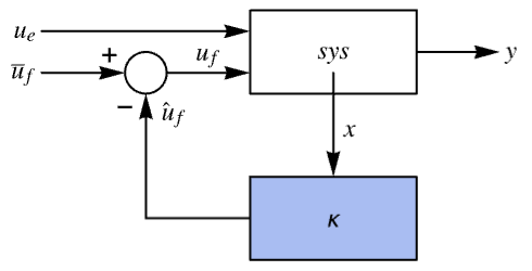
StateFeedbackGains[sys, p, {"ClosedLoopSystem", <|"Merge" -> False|>}]SystemsModelMerge[%]StateFeedbackGains[sys, p, {"ClosedLoopSystem", <|"Merge" -> True|>}]sm = CreateSystemModel["MassSpringDamper", {m x''[t] + c x'[t] + k x[t] == u[t], y[t] == x[t]}, t, {"u"∈"Modelica.Blocks.Interfaces.RealInput", "y"∈"Modelica.Blocks.Interfaces.RealOutput"}, <|"ParameterValues" -> {m -> 10, c -> 10^2, k -> 10^3}|>];csysName = "MassSpringDamperWithStateFeedback";csys = StateFeedbackGains[sm, {-2, -3}, {"ClosedLoopSystem", <|"ModelName" -> csysName|>}]csys["ModelName"]この名前を直接使って他の関数の閉ループ系のモデルが指定できる:
SystemModelSimulate[csysName, {"y"}, 10, <|"Inputs" -> {"u" -> UnitStep}|>]SystemModelPlot[%, All]オプション (6)
Method (6)
デフォルトで,厳密値または記号値を持つ系には"Ackermann"メソッドが使われる:
ssm = StateSpaceModel[{{{0, 1}, {-k/m, -c/m}},
  {{c/m}, {-c^2/m^2 +
     k/m}}, {{1, 0}}, {{0}}}, SamplingPeriod -> None,
 SystemsModelLabels -> None];
StateFeedbackGains[ssm, {Subscript[p, 1], Subscript[p, 2]}]StateFeedbackGains[ssm, {Subscript[p, 1], Subscript[p, 2]}, Method -> "Ackermann"] === %厳密ではない系には,デフォルトで,"KNVD"メソッドが使われる:
ssm = StateSpaceModel[{{{-1.2, 0.2}, {1., -4.1}}, {{2., 0}, {0., 1.}}, {{1., 1.1}}, {{0, 0}}},
 SamplingPeriod -> None, SystemsModelLabels -> None];
StateFeedbackGains[ssm, {-1., -2.}]StateFeedbackGains[ssm, {-1., -2.}, Method -> "KNVD"] === %少なくとも状態と同じだけの入力がある非厳密系にはLinearSolveが使われる:
StateFeedbackGains[StateSpaceModel[{{{a}}, {{Subscript[b, 1],
    Subscript[b, 2]}}, {{c}}, {{0, 0}}}, SamplingPeriod -> None,
SystemsModelLabels -> None], {p}, Method -> Automatic]LinearSolve[{{Subscript[b, 1], Subscript[b, 2]}}, {{a - p}}]ssm = StateSpaceModel[{{{-1.2, 0.2}, {1., -4.1}}, {{2., 0}, {0., 1.}}, {{1., 1.1}}, {{0, 0}}},
SamplingPeriod -> None, SystemsModelLabels -> None];
p = {-3 + 2 I, -3 - 2I };StateFeedbackGains[ssm, p] === StateFeedbackGains[ssm, p, Method -> "KNVD"]"Ackermann"メソッドでは多重入力系に対して1つの入力しか使われない:
ssm = StateSpaceModel[{{{-1.2, 0.2}, {1., -4.1}}, {{2., 0}, {0., 1.}}, {{1., 1.1}}, {{0, 0}}},
 SamplingPeriod -> None, SystemsModelLabels -> None];
p = {-3 + 2 I, -3 - 2I };κ = StateFeedbackGains[ssm, p, Method -> "Ackermann"]Position[κ, {0..}]Table[SingularValueList[ControllabilityMatrix[SystemsModelExtract[ssm, i]]], {i, 2}];Table[i[[1]] / i[[-1]], {i, %}]"KNVD"閉ループ極はフィードバックゲインの摂動に対して"Ackermann"ほど敏感ではない:
ssm = StateSpaceModel[{{{-10, 0, -10, 0}, {0, -0.7, 9, 0}, {0, -1, -0.7, 0}, {1, 0, 0, 0}},
  {{20, 2.8}, {0, -3.13}, {0, 0}, {0, 0}}}, SamplingPeriod -> None, SystemsModelLabels -> None];
p = {-10, -8, -5, -2};MatrixForm /@ {Subscript[κ, 1] = StateFeedbackGains[ssm, p, Method -> "KNVD"], Subscript[κ, 2] = StateFeedbackGains[ssm, p, Method -> "Ackermann"]}δp = RandomReal[{-0.1, 0.1}, Dimensions[Subscript[κ, 1]]];
MatrixForm /@ {Subscript[κ, 1] += δp, Subscript[κ, 2] += δp}csys = Table[SystemsModelStateFeedbackConnect[ssm, κ], {κ, {Subscript[κ, 1], Subscript[κ, 2]}}];
{Subscript[p, 1], Subscript[p, 2]} = Table[Eigenvalues@First@Normal[sys], {sys, csys}]指定された極からの最大誤差は"KNVD"メソッドの方が小さい:
Table[Norm[(pl - p/p), Infinity], {pl, {Subscript[p, 1], Subscript[p, 2]}}]アプリケーション (14)
力学系 (4)
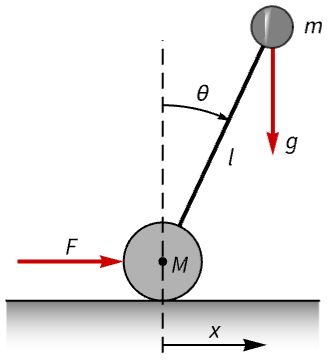
segw = NonlinearStateSpaceModel[IconizedObject[«eqns»] /. IconizedObject[«pars»], {x[t], x'[t], {θ[t], 0}, θ'[t]}, f[t], {x[t], θ[t]}, t]//Simplifyコントローラがないと,セグウェイの位置と向きのバランスが取れない:
OutputResponse[{segw, {0, 0, 0.1}}, 0, {t, 0, 10}];
Plot[%, {t, 0, 10}, PlotRange -> All, PlotLegends -> {θ, x}]segw = NonlinearStateSpaceModel[segw, Automatic, Automatic, Automatic, None];p = {-2 + 0.5I, -2 - 0.5I, -3.5, -1.5};
𝒸𝒹 = StateFeedbackGains[segw, p, "Data"]𝒸𝒹["ClosedLoopPoles"]𝒸𝒹["OpenLoopPoles"]csys = 𝒸𝒹["ClosedLoopSystem"]//FullSimplifysr = StateResponse[{csys, {0, 0, 0.1}}, 0, {t, 0, 10}];
Table[Plot[𝓈𝓇[[1]], {t, 0, 15}, IconizedObject[«plotOpts»]], {𝓈𝓇, ({sr, {θ, ω, x, x'}})}]or = OutputResponse[csys, 0.2UnitBox[t - 1], {t, 0, 20}];
Table[Plot[ℴ𝓇[[1]], {t, 0, 15}, IconizedObject[«plotOpts»]], {ℴ𝓇, ({or, {θ, x}})}]OutputResponse[𝒸𝒹["ControllerModel"], Join[{0}, sr], {t, 0, 10}];
Plot[%, {t, 0, 10}, PlotRange -> All]柔軟な接合部を備えたシングルリンクロボットマニピュレータの調整器を設計する:
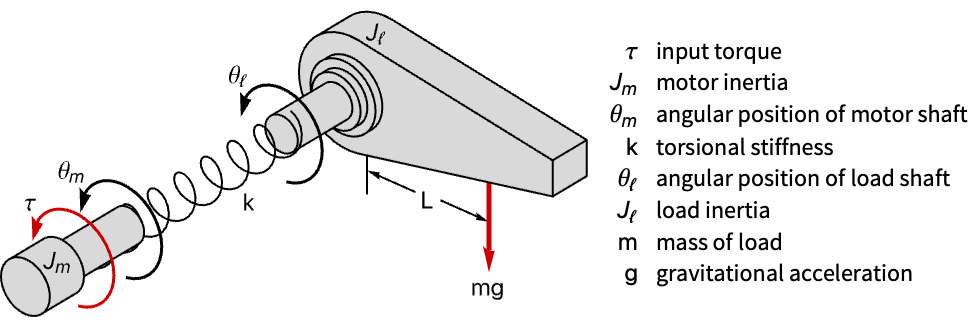
robotM = NonlinearStateSpaceModel[IconizedObject[«eqns»] /. IconizedObject[«pars»], {θ[t], θ'[t], ϕ[t], ϕ'[t]}, τ[t], θ[t], t];
robotM = NonlinearStateSpaceModel[robotM, Automatic, Automatic, Automatic, None]OutputResponse[{robotM, {0.2}}, 0, {t, 0, 15}];
Plot[%, {t, 0, 15}, PlotRange -> All]p = {-1 + I, -1 - I, -4 + 0.25I, -4 - 0.25I};
𝒸𝒹 = StateFeedbackGains[robotM, p, "Data"]csys = 𝒸𝒹["ClosedLoopSystem"]sr = StateResponse[{csys, {0.05}}, 0, {t, 0, 15}];
Table[Plot[𝓈𝓇[[1]], {t, 0, 15}, IconizedObject[«plotOpts»]], {𝓈𝓇, ({sr, {θ, θ', ϕ, ϕ'}})}]cm = 𝒸𝒹["ControllerModel"]OutputResponse[cm, Join[{0}, sr], {t, 0, 10}];
Plot[%, {t, 0, 10}, PlotRange -> All]ボールとビームの系について離散時間安定化コントローラを設計する:
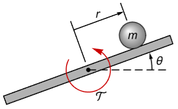
bbs = StateSpaceModel[IconizedObject[«eqns»] /. IconizedObject[«pars»], {r[t], θ[t]}, 𝒯[t], r[t], t, IconizedObject[«labels»]]
τ = 0.2;
bbd = ToDiscreteTimeModel[bbs, τ]OutputResponse[{bbd, {0, 0, 0.01}}, Table[0, 10]];
ListStepPlot[%, DataRange -> {0, 9 τ}, PlotRange -> All]p = {0.7, -0.75, 0.05 + 0.0125I, 0.05 - 0.0125I};
𝒸𝒹 = StateFeedbackGains[bbd, p, "Data"]csys = 𝒸𝒹["ClosedLoopSystem"]sr = StateResponse[{csys, {0, 0, 0.25, 0}}, Table[0, 30]];
ListStepPlot[%[[1]], DataRange -> {0, 29 τ}, PlotRange -> All]OutputResponse[𝒸𝒹["ControllerModel"], Join[{Table[0, 30]}, sr]];
ListStepPlot[%, DataRange -> {0, 29 τ}, PlotRange -> All]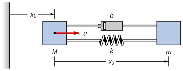
ssm = StateSpaceModel[IconizedObject[«eqns»] /. IconizedObject[«pars»], {Subscript[x, 1][t], Subscript[x, 1]'[t], Subscript[x, 2][t], Subscript[x, 2]'[t]}, u[t], {Subscript[x, 1][t], Subscript[x, 2][t]}, t, IconizedObject[«labels»]]サンプリング周期を  とし,0次ホールド法を使ってこれを離散化する:
τ = 0.4;
ssmd = ToDiscreteTimeModel[ssm, 0.4, Method -> "ZeroOrderHold"]

OutputResponse[{ssmd, {1}}, Table[0, 30]];
ListStepPlot[%, DataRange -> {0, 29 τ}, IconizedObject[«plotOpts»]]Subscript[𝒸𝒹, 1] = StateFeedbackGains[ssmd, {0.9, 0.4, 0.3, 0.1}, "Data"]Subscript[𝒸𝒹, 2] = StateFeedbackGains[ssmd, {0.75 + 0.4I, 0.75 - 0.4I, 0.1, 0.2}, "Data"]{Subscript[csys, 1], Subscript[csys, 2]} = Table[Subscript[𝒸𝒹, i]["ClosedLoopSystem"], {i, 2}]{Subscript[sr, 1], Subscript[sr, 2]} = Table[StateResponse[{Subscript[csys, i], {1}}, Table[0, 30]], {i, 2}];Table[ListStepPlot[Subscript[sr, i][[{1, 3}]], DataRange -> {0, 29τ}, IconizedObject[«plotOpts»]], {i, 2}]{Subscript[κ, 1], Subscript[κ, 2]} = Table[Subscript[𝒸𝒹, i]["FeedbackGains"], {i, 2}]Table[ListStepPlot[-Subscript[κ, i].Subscript[sr, i], PlotRange -> All, ImageSize -> Small], {i, 2}]電気機械系 (1)
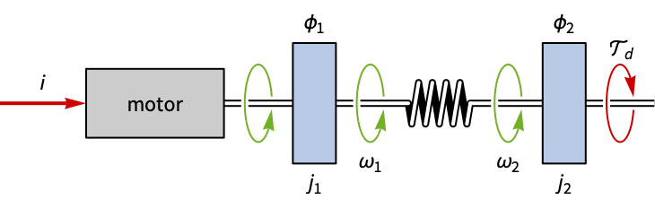
gauge = StateSpaceModel[IconizedObject[«eqns»] /. IconizedObject[«pars»], {Subscript[ϕ, 1][t], Subscript[ω, 1][t], Subscript[ϕ, 2][t], Subscript[ω, 2][t]}, {i[t] , Subscript[𝒯, d][t]}, Subscript[ϕ, 2][t], t, IconizedObject[«labels»]]OutputResponse[{gauge, {0.1, 0, -0.1}}, {0, 0}, {t, 0, 200}];
Plot[%, {t, 0, 200}, PlotRange -> All]sspec = <|"InputModel" -> gauge, "FeedbackInputs" -> 1|>;振動を減衰するための状態フィードバックコントローラを設計する:
p = {-2, -1.5, -1 + I, -1 - I};
𝒸𝒹 = StateFeedbackGains[sspec, p, "Data"]𝒸𝒹["ClosedLoopPoles"]csys = 𝒸𝒹["ClosedLoopSystem"]sr = StateResponse[{csys, {0.1, 0, -0.1}}, {0, 0}, {t, 0, 10}];
Plot[%[[4]], {t, 0, 10}, PlotRange -> All]OutputResponse[csys, {0, 0.1Sin[t]}, {t, 0, 100}];
Plot[%, {t, 0, 100}, PlotRange -> {1, -1}]cm = 𝒸𝒹["ControllerModel"]OutputResponse[cm, Join[{0}, sr], {t, 0, 10}];
Plot[%, {t, 0, 10}, IconizedObject[«plotOpts»]]航空宇宙系 (2)
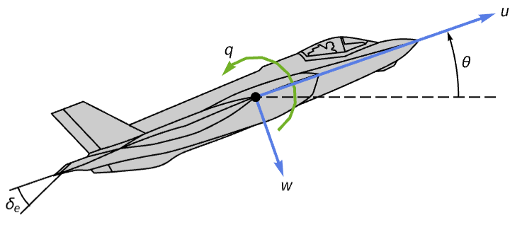
aircraft = NonlinearStateSpaceModel[IconizedObject[«eqns»] /. IconizedObject[«pars»], {u[t], w[t], q[t], θ[t]}, Subscript[δ, e][t], θ[t], t]初期摂動後にピッチ角が安定するまでにおよそ1500秒かかる:
OutputResponse[{aircraft, {0, 0, 0, 0.1}}, 0, {t, 0, 2000}];
Plot[%, {t, 0, 2000}, PlotRange -> All]aircraft = NonlinearStateSpaceModel[aircraft, Automatic, Automatic, Automatic, None];p = {-3, -1 + 0.5I, -1 - 0.5I, -1};
𝒸𝒹 = StateFeedbackGains[aircraft, p, "Data"]csys = 𝒸𝒹["ClosedLoopSystem"]sr = StateResponse[{csys, {0, 0, 0, 0.1}}, 0, {t, 0, 15}];
Table[Plot[𝓈𝓇[[1]], {t, 0, 15}, IconizedObject[«plotOpts»]], {𝓈𝓇, ({sr, {u, w, q, θ}})}]cm = 𝒸𝒹["ControllerModel"]OutputResponse[cm, Join[{0}, sr], {t, 0, 20}];Plot[%, {t, 0, 5}, PlotRange -> All]軌道を回る衛星の軌道を修正するための出力フィードバックコントローラを設計する:
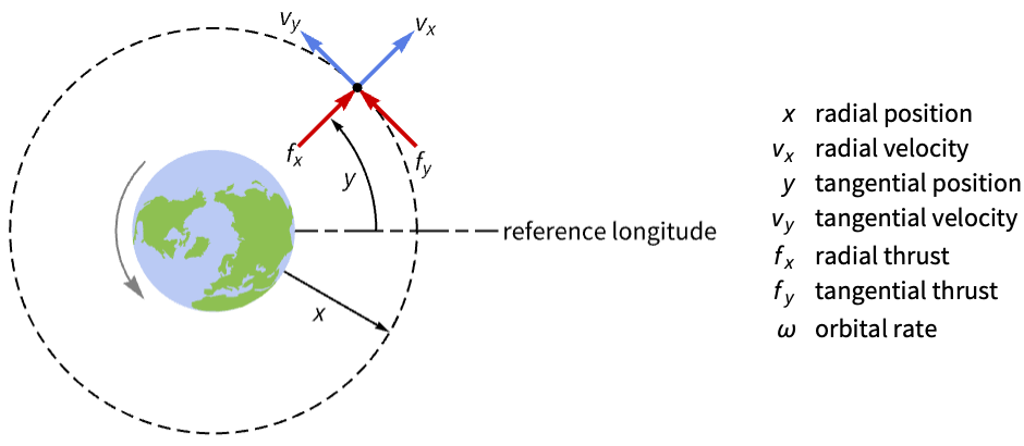
sat = StateSpaceModel[IconizedObject[«eqns»] /. ω -> 0.0011, {x[t], x'[t], y[t], y'[t]}, {Subscript[f, x][t], Subscript[f, y][t]}, {x[t], y[t]}, t, IconizedObject[«labels»]]OutputResponse[{sat, {0, 0.2, 0, 0.1}}, {0, 0}, {t, 0, 10}];
Table[Plot[%[[i]], {t, 0, 10}, IconizedObject[«plotOpts»]], {i, 2}]MatrixForm[κ = StateFeedbackGains[sat, {-0.5, -1.5, -1, -2.5}]]MatrixForm[ℓ = EstimatorGains[sat, 3 {-0.5, -1.5, -1, -2.5}]]ℯ𝓇 = EstimatorRegulator[sat, {ℓ, κ}, "Data"]csys = ℯ𝓇["ClosedLoopSystem"]//SystemsModelMergeor = OutputResponse[{csys, {0, 0.2, 0, 0.1}}, {0, 0}, {t, 0, 15}];
Plot[or, {t, 0, 15}, IconizedObject[«plotOpts»]]cm = ℯ𝓇["ControllerModel"]//SystemsModelMergeOutputResponse[cm, Join[{0}, or], {t, 0, 15}];
Plot[%, {t, 0, 15}, IconizedObject[«plotOpts»]]電気系 (3)
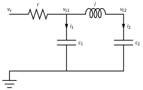
circuit = StateSpaceModel[Join[IconizedObject[«comps»], IconizedObject[«eqns»]], IconizedObject[«vars»], Subscript[v, s][t], Subscript[v, c2][t],
t, DescriptorStateSpace -> True, IconizedObject[«labels»]] /. IconizedObject[«pars»]OutputResponse[circuit, UnitStep[t], {t, 0, 10}];
Plot[%, {t, 0, 10}, PlotRange -> All, ImageSize -> Small]TransferFunctionPoles@TransferFunctionModel[circuit]//N極が減衰不足ではない状態フィードバックコントローラを設計する:
p = {-2, -5 + I, -5 - 1I};
𝒸𝒹 = StateFeedbackGains[circuit, p, "Data"]csys = 𝒸𝒹["ClosedLoopSystem"]//SystemsModelMergesr = StateResponse[csys, UnitStep[t], {t, 0, 10}];
Plot[%[[2]], {t, 0, 10}, PlotRange -> All]BodePlot[{circuit, csys}, IconizedObject[«plotOpts»]]Plot[-𝒸𝒹["FeedbackGains"].sr, {t, 0, 10}, PlotRange -> All]tfm = BiquadraticFilterModel[{"Bandpass", {{60, 5}}}, s]filter = StateSpaceModel[tfm]TransferFunctionPoles[tfm][[1, 1]]//Nフィルタの特徴を改善するためのコントローラの集合を設計する:
p = {{-6 + 50I, -6 - 50I}, {-15 + 40I, -15 - 40I}, {-25 + 30I, -25 - 30I}};
csys = Table[StateFeedbackGains[filter, 𝓅, "ClosedLoopSystem"], {𝓅, p}]or = Table[OutputResponse[sys, Sin[t], {t, 0, 2}], {sys, Join[{filter}, csys]}];
Table[Plot[ℴ𝓇[[1]], {t, 0, 2}, IconizedObject[«plotOpts»]], {ℴ𝓇, ({or, IconizedObject[«plotLabels»]})}]dcMot = StateSpaceModel[TransferFunctionModel[{{{100.23330719585297}}, 1 + 0.8*s}, s], SystemsModelLabels -> {"v", "ω"}]sspec = <|"InputModel" -> dcMot, "TrackedOutputs" -> 1|>𝒸𝒹 = StateFeedbackGains[sspec, {-1.5, -2}, "Data"]ℓ = EstimatorGains[sspec, {-3}]ℯ𝓇 = EstimatorRegulator[sspec, {ℓ, 𝒸𝒹}, "Data"]csys = ℯ𝓇["ClosedLoopSystem"]
ref = 200;
or = OutputResponse[csys, ref, {t, 0, 7}];Plot[{or, ref}, {t, 0, 7}, IconizedObject[«plotOpts»]]OutputResponse[ℯ𝓇["ControllerModel"], {ref, or[[1]]}, {t, 0, 5}]
Plot[%, {t, 0, 5}, PlotRange -> All]化学系 (2)
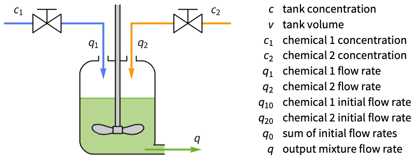
ssm = StateSpaceModel[IconizedObject[«eqns»], IconizedObject[«vars»], IconizedObject[«labels»], DescriptorStateSpace -> True] /. Subscript[q, 0] -> Subscript[q, 10] + Subscript[q, 20] /. IconizedObject[«pars»]olor = OutputResponse[ssm, {0, UnitBox[t - 1]}, {t, 0, 300}];
Plot[olor, {t, 0, 300}, PlotRange -> All]𝒸𝒹 = StateFeedbackGains[ssm, {-0.5, -0.3}, "Data"]csys = 𝒸𝒹["ClosedLoopSystem"]//Chopclsr = StateResponse[csys, {0, UnitBox[t - 1]}, {t, 0, 300}];
Plot[{olor, clsr[[3]]}, {t, 0, 300}, IconizedObject[«plotOpts»]]κ = 𝒸𝒹["FeedbackGains"]Plot[Evaluate[-κ.clsr], {t, 0, 50}, IconizedObject[«plotOpts»]]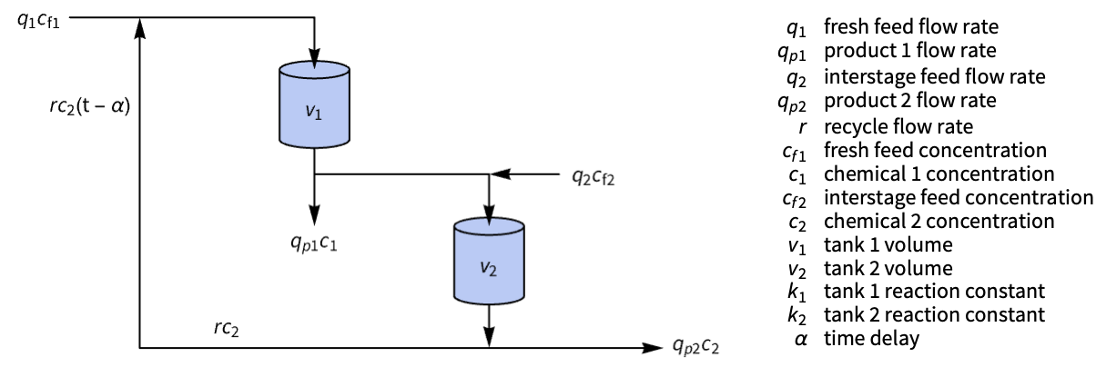
reactor = StateSpaceModel[IconizedObject[«eqns»], {Subscript[c, 1][t], Subscript[c, 2][t]}, {Subscript[c, f1][t], Subscript[c, f2][t]},
{Subscript[c, 1][t - Subscript[τ, 1]], Subscript[c, 2][t - Subscript[τ, 2]]}, t, IconizedObject[«labels»]] /. IconizedObject[«pars»]OutputResponse[{reactor, {0.1, -0.1}}, {0, 0}, {t, 0, 10}];
Plot[%, {t, 0, 10}, IconizedObject[«plotOpts»]]dfsys = MinimalStateSpaceModel[SystemsModelDelayApproximate[reactor, 0]]κ = StateFeedbackGains[dfsys, {-3 + I, -3 - I}]ℓ = EstimatorGains[dfsys, {-5, -6}]ℯ𝓇𝒻𝒷 = EstimatorRegulator[dfsys, {ℓ, κ}, "EstimatorRegulatorFeedbackModel"]smC = SmithDelayCompensator[reactor, ℯ𝓇𝒻𝒷]フィードバック経路にあるスミス補償器を持つモデルの閉ループ系を得る:
csys = SystemsModelFeedbackConnect[SystemsModelSeriesConnect[smC, reactor]]OutputResponse[{csys, {0.1, -0.1}}, {0, 0}, {t, 0, 10}];
Plot[%, {t, 0, 10}, IconizedObject[«plotOpts»]]デッドビート制御 (1)
dssm = StateSpaceModel[{{{1, 1, -2}, {0, 1, 1}, {0, 0, 1}}, {{1}, {0}, {1}}}, SamplingPeriod -> 1,
SystemsModelLabels -> None];csys = StateFeedbackGains[dssm, {0, 0, 0}, "ClosedLoopSystem"]
SystemsModelOrder[dssm]or = OutputResponse[{csys, RandomReal[{-1, 1}, 3]}, Table[0, 6]]//ChopListStepPlot[or, Right, PlotRange -> All, DataRange -> {0, 5}]海洋系 (1)
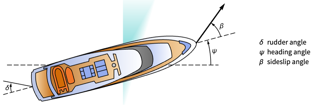
boat = StateSpaceModel[IconizedObject[«abc»], IconizedObject[«labels»]]sspec = <|"InputModel" -> boat, "TrackedOutputs" -> 1|>;cd = StateFeedbackGains[sspec, {-0.35, -0.3, -0.25 + 0.1I, -0.25 - 0.1I}, "Data"]csys = cd["ClosedLoopSystem"]Table[OutputResponse[csys, ref, {t, 0, 50}], {ref, 4, 20, 4}];
Plot[%, {t, 0, 50}, IconizedObject[«plotOpts»]]cm = cd["ControllerModel"]cinps[ref_] := Join[{ref}, OutputResponse[csys, ref, {t, 0, 50}], StateResponse[csys, ref, {t, 0, 50}][[1 ;; 3]]]Table[OutputResponse[cm, cinps[ref], {t, 0, 50}], {ref, 4, 20, 4}];
Plot[%, {t, 0, 50}, IconizedObject[«plotOpts»]]特性と関係 (17)
状態フィードバックゲインは負のフィードバックについて計算される:
a = RandomReal[{-1, 1}, {2, 2}];
b = RandomReal[{-1, 1}, {2, 1}];
p = RandomReal[{-3, -1}, 2];κ = StateFeedbackGains[StateSpaceModel[{a, b}], p]p1 = Eigenvalues[a - b.κ]ContainsExactly[p1, p, SameTest -> (Chop[#1 - #2] == 0. &)]𝒸𝒹 = StateFeedbackGains[StateSpaceModel[{{{-1, 2}, {1, 3}}, {{1}, {0}}, {{1, 0}}, {{0}}}, SamplingPeriod -> None,
SystemsModelLabels -> None], {-3, -4}, "Data"]SystemsModelStateFeedbackConnect[𝒸𝒹["InputModel"], 𝒸𝒹["FeedbackGains"]]𝒸𝒹["ClosedLoopSystem"]制御努力は閉ループ極が開ループ極から離れるにつれて大きくなる:
ssm = StateSpaceModel[{{{-3, 0}, {0, -2}}, {{1}, {-1}}}, SamplingPeriod -> None,
 SystemsModelLabels -> None];
p = {{-3, -2}, {-3, -2.5}, {-2.5, -2}, {-4, -1}, {-4, -5}};ListLinePlot[Table[{Norm[𝓅 - {-3, -2}], Norm@StateFeedbackGains[ssm, 𝓅]}, {𝓅, p}], IconizedObject[«plotOpts»]]
nsys = NonlinearStateSpaceModel[{{-2*Subscript[x, 1] + Subscript[x, 1]^2 +
    Subscript[x, 2], 1 + u - Subscript[x, 1] -
    Subscript[x, 2] + Subscript[x, 1]*Subscript[x, 2]},
  {Subscript[x, 1]}}, {{Subscript[x, 1], 1},
  {Subscript[x, 2], 1}}, {u}, {Automatic}, Automatic,
 SamplingPeriod -> None];
p = {-4 + I, -4 - I};StateFeedbackGains[nsys, p]
κ = StateFeedbackGains[StateSpaceModel[nsys], p]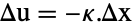
-SolveValues[{u - 1} == -κ.{Subscript[x, 1] - 1, Subscript[x, 2] - 1}, u]制御可能な標準StateSpaceModelの極はすべて状態フィードバックを使って制御できる:
ssm = StateSpaceModel[{{{0, 1}, {-1, -2}}, {{0}, {1}}, {{1, 0}}, {{0}}}, SamplingPeriod -> None,
SystemsModelLabels -> None];ControllableModelQ[ssm]p = Eigenvalues[Normal[ssm][[1]]] - RandomReal[{1, 3}, 2]cd = StateFeedbackGains[ssm, p, "Data"];
cd["FeedbackGains"]ContainsExactly[cd["ClosedLoopPoles"], p, SameTest -> (Chop[#1 - #2] == 0.&)]制御可能な非特異ディスクリプタStateSpaceModelの極もすべて制御できる:
dssm = StateSpaceModel[{{{1, 1}, {0, 0}}, {{0}, {1}}, {{3, 8}}, {{0}}, {{1, 0}, {1, 1}}},
SamplingPeriod -> None, SystemsModelLabels -> None];{ControllableModelQ[dssm], MatrixRank[Last[Normal[dssm]]]}p = Eigenvalues[Normal[dssm][[{1, -1}]]] - RandomReal[{1, 3}, 2]𝒸𝒹 = StateFeedbackGains[dssm, p, "Data"]𝒸𝒹["FeedbackGains"]ContainsExactly[𝒸𝒹["ClosedLoopPoles"], p, SameTest -> (Chop[#1 - #2] == 0.&)]制御不可能な標準StateSpaceModelの部分系のみが制御可能である:
ssm = StateSpaceModel[{{{-2., 0}, {0, -1}}, {{1}, {0}}, {{1, 1}}, {{0}}}, SamplingPeriod -> None,
 SystemsModelLabels -> None];

modes = Eigenvalues[First[Normal[ssm]]];
Table[{λ, ControllableModelQ[{ssm, {λ}}]}, {λ, modes}]

𝒸𝒹 = StateFeedbackGains[ssm, {-RandomReal[{4, 8}], -1}, "ClosedLoopPoles"]StateFeedbackGains[ssm, {-RandomReal[{4, 8}], -RandomReal[{4, 8}]}, "ClosedLoopPoles"]
非特異ディスクリプタの遅い部分系の制御可能な極だけが制御できる:
dssm = StateSpaceModel[{{{-5, 0}, {0, 1}}, {{1}, {0}}, {{1, 0}}, {{0}}, {{1, 0}, {0, 0}}},
 SamplingPeriod -> None, SystemsModelLabels -> None];
ControllableModelQ[{dssm, "Slow"}]dim = Total[Diagonal[Normal[dssm][[5]]]]p = RandomReal[{-8, -6}, dim]
𝒸𝒹 = StateFeedbackGains[dssm, p, "Data"];
𝒸𝒹["FeedbackGains"]
遅い部分系の極は希望の位置に移動され,速い部分系に対応する における極は変化しない:
{𝒸𝒹["OpenLoopPoles"], 𝒸𝒹["ClosedLoopPoles"]}{ControllableModelQ[dssm], SystemsModelOrder[dssm]}非特異ディスクリプタの制御可能な遅い部分系の極はどれも制御できない:
dssm = StateSpaceModel[{{{-5, 0}, {0, 1}}, {{0}, {0}}, {{1, 0}}, {{0}}, {{1, 0}, {0, 0}}},
 SamplingPeriod -> None, SystemsModelLabels -> None];
ControllableModelQ[{dssm, "Slow"}]dim = Total[Diagonal[Normal[dssm][[5]]]]p = RandomReal[{-8, -6}, dim]StateFeedbackGains[dssm, p, {"OpenLoopPoles", "ClosedLoopPoles"}]
LQRegulatorGainsとStateFeedbackGainsは単一入力の系に対して同じ結果を返す:
ssm = StateSpaceModel[{{{0, 1}, {-2, -0.5}}, {{0}, {1}}, {{1, 0}}, {{0}}}, SamplingPeriod -> None,
 SystemsModelLabels -> None];
𝒸𝒹 = LQRegulatorGains[ssm, {(|   |   |
| - | - |
| 2 | 0 |
| 0 | 1 |), (1)}, "Data"];LQRegulatorGains設計の閉ループ曲があるStateFeedbackGains:
StateFeedbackGains[ssm, 𝒸𝒹["ClosedLoopPoles"]]LQRegulatorGainsは同じゲインを与える:
𝒸𝒹["FeedbackGains"] ρ c.c x(t)2+u(t)2t を最小化する閉ループ極は対称根軌跡プロットを使って得ることができる:
ssm = StateSpaceModel[{{{-2, 0, 0}, {1, 0, 0}, {0, 1, 0}}, {{1}, {0}, {0}}, {{0, 0, 1}}, {{0}}},
SamplingPeriod -> None, SystemsModelLabels -> {u, y}];symTFM = With[{tfm = TransferFunctionModel[ssm, s]}, tfm[s] tfm[-s]][[1, 1]];
symRLPlot = RootLocusPlot[ρ symTFM, {ρ, 0, 20}]
p = Cases[symRLPlot, Tooltip[{___, Point[{{x_ ? Negative, y_}}]}, ρ == 10.] :> x + I y, {0, Infinity}]StateFeedbackGains[ssm, p, "FeedbackGains"]LQRegulatorGainsを使っても同じゲインが得られる:
c = Normal[ssm][[3]];
LQRegulatorGains[ssm, {10 c.c, {{1.}}}, "FeedbackGains"]StateSpaceModelについては,StateFeedbackGainsとFullInformationOutputRegulatorは同じ結果を与える:
ssm = StateSpaceModel[{{{2, 0, -1}, {0, -2, 1}, {1, -1, 1}}, {{1, 1}, {0, 1}, {1, -1}},
{{1, -1, 0}, {0, 1, -1}}, {{0, 0}, {0, 0}}}, SamplingPeriod -> None, SystemsModelLabels -> None];p = {-1, -2, -3};StateFeedbackGains[ssm, p] === FullInformationOutputRegulator[ssm, p]推定器調整器は状態フィードバック行列と推定器ゲイン行列を使って組み立てられる:
ssm  = StateSpaceModel[{{{0, 1, 0}, {0, 0, -1}, {0, 0, 0.5}}, {{0}, {1}, {1}}, {{1, 2, 4}}, {{0}}},
SamplingPeriod -> 1, SystemsModelLabels -> None];{ℓ, κ} = {EstimatorGains[ssm, {-1, -1 + I, -1 - I}], StateFeedbackGains[ssm, {-1, -1 + I, -1 - I}]}er = EstimatorRegulator[ssm, {ℓ, κ}]単一入力系の閉ループ系におけるゲインに相当する状態フィードバックゲイン:

κ = RandomReal[{0, 10}];
tfm = TransferFunctionModel[{{{k}}, (1 + s)*(2 + s)*
(3 + s)}, s];Subscript[p, cl] = TransferFunctionPoles[SystemsModelFeedbackConnect[tfm /. k -> κ]][[1, 1]]ssm = StateSpaceModel[tfm, StateSpaceRealization -> "ControllableCompanion"]この実現について,状態フィードバックゲインは{{κ,0,…,0}}の形である:
Chop[StateFeedbackGains[ssm, Subscript[p, cl]]] == {{κ, 0, 0}}κ = RandomReal[{0, 10}];
tfm = TransferFunctionModel[{{{k}}, (1 + s)*(2 + s)*
(3 + s)}, s];Subscript[p, cl] = TransferFunctionPoles[SystemsModelFeedbackConnect[tfm /. k -> κ]][[1, 1]]ssm = StateSpaceModel[tfm, StateSpaceRealization -> "ControllableCompanion"]この実現について,状態フィードバックゲインは{{κ,0,…,0}}の形である:
Chop[StateFeedbackGains[ssm, Subscript[p, cl]]] == {{κ, 0, 0}}状態フィードバックと推定器ゲインは互いに互いのデュアルである:
{ssm = StateSpaceModel[{{{0, 1, 0, 0}, {0, 0, -1, 0}, {0, 0, 0, 1}, {0, 0, 11, 0}}, {{0}, {1}, {0}, {1}},
{{1, 2, 3, 4}}, {{0}}}, SamplingPeriod -> None, SystemsModelLabels -> None], dualssm = DualSystemsModel[ssm]}p = {-1, -2, -1 + I, -1 - I};
κ = StateFeedbackGains[ssm, p]ℓ = EstimatorGains[dualssm, p]状態フィードバックゲイン行列は推定器ゲイン行列の共役転置であり,逆もまた真である:
{κ == ℓ, ℓ == κ}状態フィードバックは系の入力ブロッキング特性を変えはしない:
ssm = StateSpaceModel[{{{0, 1, 0}, {0, 0, 1}, {-1, -2, -2}}, {{0}, {0}, {1}}, {{4, 0, 1}}, {{0}}},
SamplingPeriod -> None, SystemsModelLabels -> None];TransferFunctionZeros[TransferFunctionModel[ssm]]csys = StateFeedbackGains[ssm, {-3 + 2 I, -3 - 2 I, -7}, "ClosedLoopSystem"]開ループ系も閉ループ系も入力Sin[2t]をブロックする:
or = Table[OutputResponse[sys, Sin[2t], t], {sys, {ssm, csys}}];
{Plot[or[[1]], {t, 0, 15}, IconizedObject[«plotOpts»]], Plot[or[[2]], {t, 0, 3}, IconizedObject[«plotOpts»]]}
状態フィードバックが極と零点を同じにするなら,閉ループ系は観測不能になる:
ssm = StateSpaceModel[{{{0, 1}, {-12, -8.}}, {{0}, {1}}, {{4, 1}}, {{0}}}, SamplingPeriod -> None,
SystemsModelLabels -> None];z = TransferFunctionZeros[TransferFunctionModel[ssm]]//Flattenp = {z[[1]], -8};
csys = StateFeedbackGains[ssm, p, "ClosedLoopSystem"]ObservableModelQ[csys]考えられる問題 (5)
ssm = StateSpaceModel[{{{-1, 0}, {0, -3}}, {{1}, {0}}, {{1, 2}}, {{0}}}, SamplingPeriod -> None,
 SystemsModelLabels -> None];
ControllableModelQ[ssm]StateFeedbackGains[ssm, {-4, -5}]
dssm = StateSpaceModel[{{{-5, 0}, {0, 1}}, {{0}, {0}}, {{1, 0}}, {{0}}, {{1, 0}, {0, 0}}},
 SamplingPeriod -> None, SystemsModelLabels -> None];
{ControllableModelQ[dssm], ControllableModelQ[{dssm, "Slow"}]}dim = Total[Diagonal[Normal[dssm][[5]]]]StateFeedbackGains[dssm, RandomReal[{-8, -6}, dim], {"OpenLoopPoles", "ClosedLoopPoles"}]
StateFeedbackGains[StateSpaceModel[{{{-3, 0}, {0, 2}}, {{1}, {0}}}, SamplingPeriod -> None, SystemsModelLabels -> None], RandomInteger[{-10, -1}, 2]]
KNVDメソッドは状態よりも入力の方が少ない厳密な系は処理できない:
ssm = StateSpaceModel[{{{-1, 0, 1}, {-3, 1, 2}, {1, -1, 2}}, {{1, 0}, {0, 1}, {1, -2}}},
SamplingPeriod -> None, SystemsModelLabels -> None];p = {-5 + I, -5 - I, -6};
κ = StateFeedbackGains[ssm, p, Method -> "KNVD"]
StateFeedbackGains[ssm//N, p, Method -> "KNVD"]StateFeedbackGains[ssm, p, Method -> "Ackermann"]KNVDメソッドはコンピュータシステムによって異なるゲイン集合を返すかもしれない:
ssm = StateSpaceModel[{{{0, 2, 0, 0, -2, 0}, {1, 0, 0, 0, 0, -1}, {0, 1, 0, 0, 0, 0}, {0, 0, 0, 3, 0, 0},
   {2, 0, 0, 1, 0, 0}, {0, 0, -1, 0, 1, 0}}, {{1, 2}, {0, 0}, {0, 1}, {0, -1}, {0, 1}, {0, 0}}},
 SamplingPeriod -> None, SystemsModelLabels -> None];
p = {-1, -2, -3, -4, -5, -7};{$SystemID, Subscript[κ, 1] = StateFeedbackGains[ssm//N, p, Method -> "KNVD"]}{$SystemID, Subscript[κ, 2] = StateFeedbackGains[ssm//N, p, Method -> "KNVD"]}{$SystemID, With[{ssN = Normal[ssm]}, Eigenvalues[ssN[[1]] - ssN[[2]].Subscript[κ, 1]]]}{$SystemID, With[{ssN = Normal[ssm]}, Eigenvalues[ssN[[1]] - ssN[[2]].Subscript[κ, 2]]]}テキスト
Wolfram Research (2010), StateFeedbackGains, Wolfram言語関数, https://reference.wolfram.com/language/ref/StateFeedbackGains.html (2021年に更新).
CMS
Wolfram Language. 2010. "StateFeedbackGains." Wolfram Language & System Documentation Center. Wolfram Research. Last Modified 2021. https://reference.wolfram.com/language/ref/StateFeedbackGains.html.
APA
Wolfram Language. (2010). StateFeedbackGains. Wolfram Language & System Documentation Center. Retrieved from https://reference.wolfram.com/language/ref/StateFeedbackGains.html