LinearSolve[m,b]
finds an x that solves the matrix equation m.x==b.
LinearSolve[m]
generates a LinearSolveFunction[…] that can be applied repeatedly to different b.
LinearSolve[a,b]
finds an x that solves the array equation a.x==b.


LinearSolve
LinearSolve[m,b]
finds an x that solves the matrix equation m.x==b.
LinearSolve[m]
generates a LinearSolveFunction[…] that can be applied repeatedly to different b.
LinearSolve[a,b]
finds an x that solves the array equation a.x==b.
Details and Options


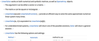
- LinearSolve works on both numerical and symbolic matrices, as well as SparseArray objects.
- The argument b can be either a vector or a matrix. »
- The matrix m can be square or rectangular. »
- LinearSolve[m] and LinearSolveFunction[…] provide an efficient way to solve the same approximate numerical linear system many times.
- LinearSolve[m,b] is equivalent to LinearSolve[m][b].
- For underdetermined systems, LinearSolve will return one of the possible solutions; Solve will return a general solution. »
- For an n1×…×nk×m array a and an n1×…×nk×d1×…×dl array b, LinearSolve[a,b] gives an m×d1×…×dl array x, such that a.xb.
- LinearSolve has the following options and settings:
-
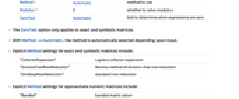
Method Automatic method to use Modulus 0 prime modulus to use ZeroTest Automatic test to determine when expressions are zero - LinearSolve[m,…Modulusp] solves rational systems modulo the prime p. If p is zero, ordinary arithmetic is used. »
- The ZeroTest option only applies to exact and symbolic matrices.
- With Method->Automatic, the method is automatically selected depending upon input.
- Explicit Method settings for exact and symbolic matrices include:
-
"CofactorExpansion" Laplace cofactor expansion "DivisionFreeRowReduction" Bareiss method of division-free row reduction "OneStepRowReduction" standard row reduction - Explicit Method settings for approximate numeric matrices include:
-
"Banded" banded matrix solver "Cholesky" Cholesky method for positive definite Hermitian matrices "Krylov" iterative Krylov sparse solver "Multifrontal" direct sparse LU decomposition "Mumps" parallel direct sparse solver "Pardiso" parallel direct sparse solver
Examples
open all close allBasic Examples (3)
Scope (16)
Basic Uses (9)
Solve a case where ![]() is a matrix:
is a matrix:
Find a solution for an exact, rectangular matrix:
Compute a solution at arbitrary precision:
Solve the system when ![]() is a matrix:
is a matrix:
Solve ![]() for CenteredInterval matrices:
for CenteredInterval matrices:
Find random representatives mrep and brep of m and b:
Verify that sol contains LinearSolve[mrep,brep]:
Solve ![]() for
for ![]() when
when ![]() is a matrix of different dimensions:
is a matrix of different dimensions:
When no right‐hand side ![]() for
for ![]() is given, a LinearSolveFunction is returned:
is given, a LinearSolveFunction is returned:
This contains data to solve the problem quickly for a few values of ![]() :
:
Special Matrices (6)
As the result is typically not sparse, the result is returned as an ordinary list:
Sparse methods are used to efficiently solve sparse matrices:
Solve a system with structured matrices:
Use a different type of matrix structure:
An identity matrix always produces a trivial solution:
Solve a linear system whose coefficient matrix is a Hilbert matrix:
Solve a ![]() system whose coefficients are univariate polynomials of degree
system whose coefficients are univariate polynomials of degree ![]() :
:
Options (7)
Method (6)
"Cholesky" (1)
"Krylov" (2)
The following suboptions can be specified for the method "Krylov":
| "BasisSize" | the size of the Krylov basis (GMRES only) | |
| "MaxIterations" | the maximum number of iterations | |
| "Method" | methods to be used | |
| "Preconditioner" | which preconditioner to apply | |
| "PreconditionerSide" | how to apply a preconditioner ("Left" or "Right") | |
| "ResidualNormFunction" | A norm function that computes a norm of the residual of the solution | |
| "StartingVector" | the initial vector to start iterations | |
| "Tolerance" | the tolerance used to terminate iterations |
Possible settings for "Method" include:
| "BiCGSTAB" | iterative method for arbitrary square matrices | |
| "ConjugateGradient" | iterative method for Hermitian positive definite matrices | |
| "GMRES" | iterative method for arbitrary square matrices |
Possible settings for "Preconditioner" include:
| "ILU0" | a preconditioner based on an incomplete LU factorization of the original matrix without fill-in | |
| "ILUT" | a variant of ILU0 with fill-in | |
| "ILUTP" | a variant of ILUT with column permutation |
Possible suboptions for "Preconditioner" include:
| "FillIn" | upper bound on the number of additional nonzero elements in a row introduced by the ILUT preconditioner | |
| "PermutationTolerance" | when to permute columns | |
| "Tolerance" | drop tolerance (any element of magnitude smaller than this tolerance is treated as zero) |
"Multifrontal" (1)
Applications (11)
Spans and Linear Independence (3)
The following three vectors are not linearly independent:
The equation with a generic right-hand side does not have a solution:
Equivalently, the equation with the identity matrix on the right-hand side has no solution:
The following three vectors are linearly independent:
The equation with a generic right-hand side has a solution:
Equivalently, the equation with the identity matrix on the right-hand side has a solution:
The solution is the inverse of ![]() :
:
Determine if the following vectors are linearly independent or not:
As ![]() does not have a solution for an arbitrary
does not have a solution for an arbitrary ![]() , they are not linearly independent:
, they are not linearly independent:
Equation Solving and Invertibility (6)
Solve the following system of equations:
Rewrite the system in matrix form:
Use LinearSolve to find a solution:
Show that the solution is unique using NullSpace:
Verify the result using SolveValues:
Find all solutions of the following system of equations:
First, write the coefficient matrix ![]() , variable vector
, variable vector ![]() and constant vector
and constant vector ![]() :
:
LinearSolve gives a particular solution:
NullSpace gives a basis for solutions to the homogeneous equation ![]() :
:
Define ![]() to be an arbitrary linear combination of the elements of
to be an arbitrary linear combination of the elements of ![]() :
:
The general solution is the sum of ![]() and
and ![]() :
:
Determine if the following matrix has an inverse:
Since the system ![]() has no solution,
has no solution, ![]() does not have an inverse:
does not have an inverse:
Verify the result using Inverse:
Determine if the following matrix has a nonzero determinant:
Since the system ![]() has a solution,
has a solution, ![]() 's determinant must be nonzero:
's determinant must be nonzero:
Confirm the result using Det:
Find the inverse of the following matrix:
To find the inverse, first solve the system ![]() :
:
Verify the result using Inverse:
Solve the system ![]() , with several different
, with several different ![]() by means of computing a LinearSolveFunction:
by means of computing a LinearSolveFunction:
Perform the computation by inverting the matrix and multiplying by the inverse:
The results are practically identical, even though LinearSolveFunction is multiple times faster:
Calculus (2)
Newton's method for finding a root of a multivariate function:
Compare with the answer found by FindRoot:
Approximately solve the boundary value problem ![]() using discrete differences:
using discrete differences:
Properties & Relations (9)
For an invertible matrix ![]() , LinearSolve[m,b] gives the same result as SolveValues for the corresponding system of equations:
, LinearSolve[m,b] gives the same result as SolveValues for the corresponding system of equations:
Create the corresponding system of linear equations:
Confirm that SolveValues gives the same result:
LinearSolve always returns the trivial solution ![]() to the homogenous equation
to the homogenous equation ![]() :
:
Use NullSpace to get the complete spanning set of solutions if ![]() is singular:
is singular:
Compare with the result of SolveValues:
If ![]() is nonsingular, the solution
is nonsingular, the solution ![]() of
of ![]() is the inverse of
is the inverse of ![]() when
when ![]() is the identity matrix:
is the identity matrix:
In this case there is no solution to ![]() :
:
Use LeastSquares to minimize ![]() :
:
Compare to general minimization:
If ![]() can be solved, LeastSquares is equivalent to LinearSolve:
can be solved, LeastSquares is equivalent to LinearSolve:
For a square matrix, LinearSolve[m,b] has a solution for a generic b iff Det[m]!=0:
For a square matrix, LinearSolve[m,b] has a solution for a generic b iff m has full rank:
For a square matrix, LinearSolve[m,b] has a solution for a generic b iff m has an inverse:
For a square matrix, LinearSolve[m,b] has a solution for a generic b iff m has a trivial null space:
Possible Issues (4)
Solution found for an underdetermined system is not unique:
All solutions are found by Solve:
LinearSolve gave the solution corresponding to ![]() :
:
With ill-conditioned matrices, numerical solutions may not be sufficiently accurate:
The solution is more accurate if sufficiently high precision is used:
Some of the linear solvers available are not deterministic. Set up a system of equations:
The "Pardiso" solver is not deterministic:
The Automatic solver method is deterministic:
LinearSolve may not give a result if a non-prime Modulus is provided:
Related Guides
Related Links
History
Introduced in 1988 (1.0) | Updated in 1996 (3.0) ▪ 2003 (5.0) ▪ 2014 (10.0) ▪ 2022 (13.2) ▪ 2023 (13.3) ▪ 2024 (14.0) ▪ 2024 (14.1)
Text
Wolfram Research (1988), LinearSolve, Wolfram Language function, https://reference.wolfram.com/language/ref/LinearSolve.html (updated 2024).
CMS
Wolfram Language. 1988. "LinearSolve." Wolfram Language & System Documentation Center. Wolfram Research. Last Modified 2024. https://reference.wolfram.com/language/ref/LinearSolve.html.
APA
Wolfram Language. (1988). LinearSolve. Wolfram Language & System Documentation Center. Retrieved from https://reference.wolfram.com/language/ref/LinearSolve.html
BibTeX
@misc{reference.wolfram_2025_linearsolve, author="Wolfram Research", title="{LinearSolve}", year="2024", howpublished="\url{https://reference.wolfram.com/language/ref/LinearSolve.html}", note=[Accessed: 06-May-2026]}
BibLaTeX
@online{reference.wolfram_2025_linearsolve, organization={Wolfram Research}, title={LinearSolve}, year={2024}, url={https://reference.wolfram.com/language/ref/LinearSolve.html}, note=[Accessed: 06-May-2026]}