



StateFeedbackGains
StateFeedbackGains[sspec,{p1,…,pn}]
给出系统规范 sspec 的状态反馈增益,以将其闭环极点置于 pi.
StateFeedbackGains[…,"prop"]
给出属性值 "prop".
更多信息和选项
- StateFeedbackGains 也称为极点放置增益或特征值放置.
- StateFeedbackGains 用于计算调节控制器或跟踪控制器.
- StateFeedbackGains 通过将闭环系统极点修改为位于 pi 位置起作用.
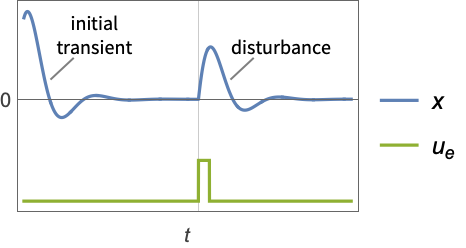
- 调节控制器旨在在尽管有扰动
 将其推开的情况下将系统保持在平衡状态. 典型范例包括将倒立摆保持在直立位置或保持飞机水平飞行.
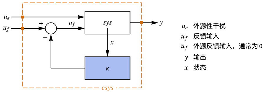
- 调节控制器由
 形式的控制律给出,其中
 是计算得到的增益矩阵.
- 要放置的极点数 n 由系统 sys 的 SystemsModelOrder 给出.
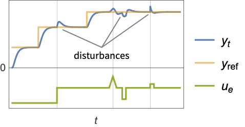
- 跟踪控制器旨在尽管有扰动
 干扰的情况下跟踪参考信号. 典型范例包括汽车的巡航控制系统或机器人的路径跟踪.
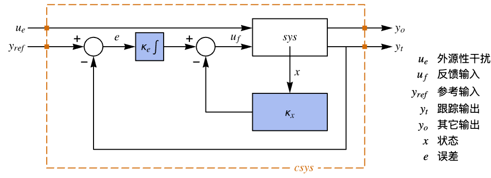
- 跟踪控制器由形式为
 的控制律给出,其中
 是为增强系统计算的增益矩阵,包括系统 sys 以及
 .
- 要放置的极点数 n 由
 给出,其中
 由 sys 的 SystemsModelOrder 给出,
 是 yref 的阶数,
 是 yref 的信号数.
- 极点放置适用于 StateSpaceModel 指定的线性系统:
-

连续时间系统 
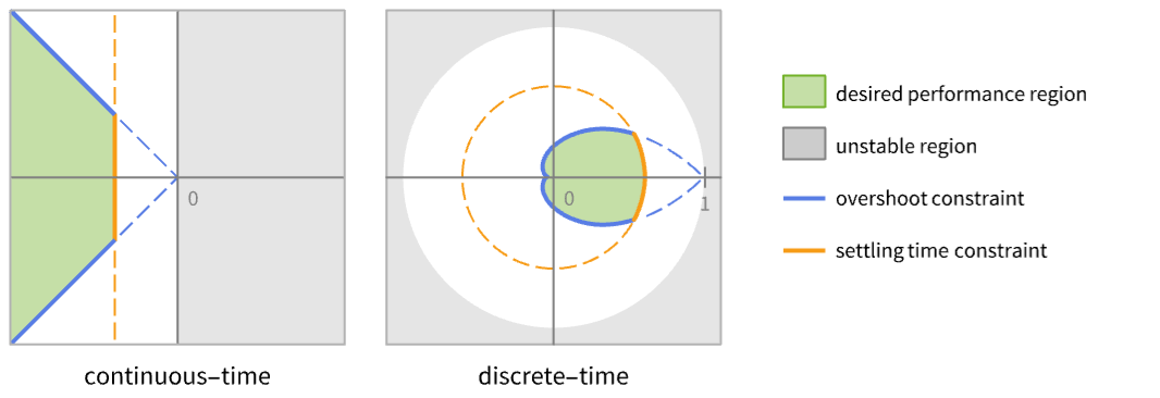
离散时间系统 - 所得闭环系统 csys 的性能主要取决于极点 pi 的位置.
- 通常存在诸如稳定时间之类的性能限制和诸如过冲之类的质量限制. 这些对应于理想的极点位置的某些区域.
- 系统规范 sspec 是系统 sys 以及 uf、yt 和 yref 规范.
- 系统规范 sspec 可以有以下形式:
-
StateSpaceModel[…] 线性控制输入和线性状态 AffineStateSpaceModel[…] 线性控制输入和非线性状态 NonlinearStateSpaceModel[…] 非线性控制输入和非线性状态 SystemModel[…] 一般系统模型 <…> 以 Association 形式给出的详细系统规范 - 详细的系统规范可以有以下密钥:
-
"InputModel" sys 任一模型 "FeedbackInputs" All 反馈输入 uf "TrackedOutputs" None 跟踪输出 yt "TrackedSignal" Automatic yref 的动态 - 跟踪信号动态作为参考信号和时间变量的函数给出. 默认情况下,假定其为常数.
-
Function[{r, t},r'[t]] 连续时间系统 Function[{r,k},r[k+1]-r[k]] 离散时间系统 - 反馈输入和跟踪输出可以有以下形式:
-
{num1,…,numn} StateSpaceModel、AffineStateSpaceModel 和 NonlinearStateSpaceModel 使用的有编号输入 numi {name1,…,namen} SystemModel 使用的有名称输入 namei All 使用所有输入 - 对于诸如 AffineStateSpaceModel、NonlinearStateSpaceModel 和 SystemModel,等非线性系统,系统将围绕其存储的工作点进行线性化.
- StateFeedbackGains[…,"Data"] 返回一个 SystemsModelControllerData 对象 cd,该对象可用于使用 cd["prop"] 形式提取其他属性.
- StateFeedbackGains[…,"prop"] 可用于直接获取 cd["prop"] 的值.
- 属性 "prop" 的可能值包括:
-
"BlockDiagram" csys 的框图 {"BlockDiagram",<"SampledData"True>} 创建 csys 的采样数据框图 "ClosedLoopPoles" 经线性化 "ClosedLoopSystem" 的极点 "ClosedLoopSystem" 系统 csys {"ClosedLoopSystem", cspec} 对闭环系统形式的详细控制 "ControllerModel" 模型 cm "Design" 控制器设计类型 "DesignModel" 用于设计的模型 "FeedbackGains" 增益矩阵 κ 或其等价物 "FeedbackGainsModel" 模型 gm 或 {gm1,gm2} "FeedbackInputs" 用于反馈的 sys 的输入 uf "InputModel" 输入模型 sys "InputCount" sys 的输入 u 的数量 "OpenLoopPoles" "DesignModel" 的极点 "OutputCount" 系统的输出 y 的数量 "SamplingPeriod" sys 的采样周期 "StateCount" sys 的状态数量 x "TrackedOutputs" 被追踪的 sys 的输出 yt - cspec 的可能密钥包括:
-
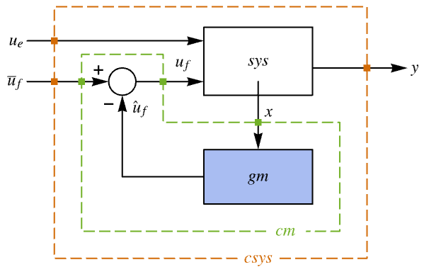
"InputModel" csys 中的输入模型 "Merge" 是否合并 csys "ModelName" csys 的名称Null "SamplingPeriod" 创建采样数据 csys - 稳压器布局图.
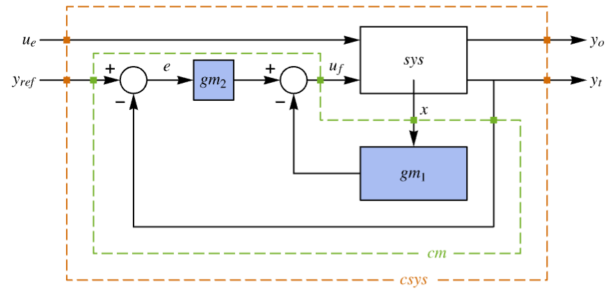
- 跟踪器布局图.
- StateFeedbackGains 接受 Method 选项,其中设置由下面任何一个给出:
-
Automatic 自动选择方法 "Ackermann" Ackermann 方法 "KNVD" Kautsky–Nichols–Van Dooren 方法
范例
打开所有单元 关闭所有单元基本范例 (3)
有反馈 uf 和外生输入 ue 的系统规格 sspec 的反馈增益:
sspec = <|"InputModel" -> StateSpaceModel[{{{0, 1}, {1, 2}}, {{1, 0}, {1, 2}}, {{0, 1}}, {{0, 0}}}, SamplingPeriod -> None,
SystemsModelLabels -> {{uf, ue}}], "FeedbackInputs" -> 1|>;p = {-4 + 3I, -4 - 3I};StateFeedbackGains[sspec, p]nsys = NonlinearStateSpaceModel[{{-1 + Subscript[x, 2],
u + Subscript[x, 1] - 2*Subscript[x, 2]},
{Subscript[x, 1] + Subscript[x, 2]}},
{{Subscript[x, 1], 1}, {Subscript[x, 2], 1}}, {{u, 1}},
{Automatic}, Automatic, SamplingPeriod -> None];p = {-2 + I, -2 - I};StateFeedbackGains[nsys, p]StateFeedbackGains[StateSpaceModel[nsys], {-2 + I, -2 - I}]𝒸𝒹 = StateFeedbackGains[StateSpaceModel[{{{0, 5}, {-1, 2.5}}, {{0}, {1}}, {{1, 1}}, {{0}}}, SamplingPeriod -> None,
SystemsModelLabels -> None], {-2, -1.5}, "Data"]PoleZeroPlot[Table[𝒸𝒹[prop], {prop, {"InputModel", "ClosedLoopSystem"}}], IconizedObject[«plotOpts»]]范围 (34)
基本用法 (8)
ssm = StateSpaceModel[{{{a}}, {{b}}, {{c}}, {{d}}},
SamplingPeriod -> None, SystemsModelLabels -> None];κ = StateFeedbackGains[ssm, {p}]SystemsModelStateFeedbackConnect[ssm, κ]ssm = StateSpaceModel[{{{2}}, {{1}}, {{1}}, {{0}}}, SamplingPeriod -> None, SystemsModelLabels -> None];κ = StateFeedbackGains[ssm, {-1}]
csys = SystemsModelStateFeedbackConnect[ssm, κ]Table[Expand[OutputResponse[sys, 1, t]], {sys, {ssm, csys}}];ssm = StateSpaceModel[{{{0, 1}, {-1, -2}}, {{0}, {1}}, {{1, 0}}, {{0}}}, SamplingPeriod -> None,
SystemsModelLabels -> None];κ = StateFeedbackGains[ssm, {-2, -3}]Dimensions[κ]ssm = StateSpaceModel[{{{0, 0, -0.1}, {1., 0., -1.08}, {0., 1., -0.9}}, {{1, 1}, {1, 0}, {0, 0}},
{{0, 0, 1}}, {{0, 0}}}, SamplingPeriod -> None, SystemsModelLabels -> None];StateFeedbackGains[ssm, {-1, -2, -2.5}]//MatrixFormssm = StateSpaceModel[{{{0, 1}, {-2, -3}}, {{0}, {1}}, {{2, 0}}, {{0}}}, SamplingPeriod -> None,
SystemsModelLabels -> None];StateFeedbackGains[ssm, {-2 + I , -2 - I}]StateFeedbackGains[ssm, {-2 , -2 - I}]ssm = StateSpaceModel[{{{0, 0, -0.1}, {1., 0., -1.08}, {0., 1., -0.9}}, {{1, 1}, {1, 0}, {0, 0}},
{{0, 0, 1}}, {{0, 0}}}, SamplingPeriod -> None, SystemsModelLabels -> None];StateFeedbackGains[ssm, {-1 + I , -1 - I, -2}]如果极点不是复共轭的,则控制将是复数并且仅使用其中一个输入:
κ = StateFeedbackGains[ssm, {-1 + I , -1, -2}]Position[κ, {0..}]ssm = StateSpaceModel[{{{0, 0, -0.1}, {1., 0., -1.08}, {0., 1., -0.9}}, {{1, 1}, {1, 0}, {0, 0}},
{{0, 0, 1}}, {{0, 0}}}, SamplingPeriod -> None, SystemsModelLabels -> None];
p = {-1 + I , -1 - I, -2};StateFeedbackGains[<|"InputModel" -> ssm, "FeedbackInputs" -> {1}|>, p]StateFeedbackGains[<|"InputModel" -> ssm, "FeedbackInputs" -> {2}|>, p]StateFeedbackGains[<|"InputModel" -> ssm, "FeedbackInputs" -> {1, 2}|>, p]assm = AffineStateSpaceModel[{{E^(1 - Subscript[x, 1]) + Subscript[x, 2],
Subscript[x, 1] - Subscript[x, 2]},
{{Subscript[x, 1]}, {0}}, {Subscript[x, 1]}, {{0}}},
{{Subscript[x, 1], 1}, {Subscript[x, 2], 1}}, {{u, -2}},
{Automatic}, Automatic, SamplingPeriod -> None]StateFeedbackGains[assm, {-2, -3}]StateFeedbackGains[StateSpaceModel[assm], {-2, -3}]工厂模型 (6)
连续时间 StateSpaceModel:
StateFeedbackGains[StateSpaceModel[{{{0, 1.}, {-1, -1.6}}, {{0}, {1}}, {{1, 1}}, {{0}}}, SamplingPeriod -> None,
SystemsModelLabels -> None], {-1.5 + I, -1.5 - I}]离散时间 StateSpaceModel:
StateFeedbackGains[StateSpaceModel[{{{0, 1.}, {0.020000000000000004, 0.1}}, {{0}, {1}}, {{1, 0}}, {{0}}},
SamplingPeriod -> τ, SystemsModelLabels -> None], {0, 0.1}]描述符 StateSpaceModel:
StateFeedbackGains[StateSpaceModel[{{{-6, -4}, {-6, -5}}, {{1}, {1}}, {{1, 0}}, {{0}}, {{1, 1}, {0, 1}}},
{{x1[t], 0}, {x2[t], 0}},
{{u[t], 0}}, Automatic, t, SamplingPeriod -> None,
SystemsModelLabels -> None], {-2.5, -3}]没有运行点的 AffineStateSpaceModel 被视作 0:
StateFeedbackGains[AffineStateSpaceModel[{{Sin[Subscript[x, 1]] + Subscript[x, 2],
-Subscript[x, 1] - Subscript[x, 2]},
{{Subscript[x, 1]}, {1}}, {Subscript[x, 1]}, {{0}}},
{Subscript[x, 1], Subscript[x, 2]}, {{u, 0}}, {Automatic},
Automatic, SamplingPeriod -> None], {-2, -3}]没有运行点的 NonlinearStateSpaceModel 被视作 0:
StateFeedbackGains[NonlinearStateSpaceModel[
{{Subscript[x, 2] + Subscript[x, 1]*Subscript[x, 2],
u + Subscript[x, 1]}, {Subscript[x, 1]}},
{Subscript[x, 1], Subscript[x, 2]}, {u}, {Automatic},
Automatic, SamplingPeriod -> None], {-1, -2}]sm = CreateSystemModel[{x''[t] + x'[t] + x[t] == 2 u[t], y[t] == x[t]}, t, {"u"∈"Modelica.Blocks.Interfaces.RealInput", "y"∈"Modelica.Blocks.Interfaces.RealOutput"}];StateFeedbackGains[sm, {-1, -2}]属性 (12)
StateFeedbackGains 默认返回反馈增益:
ssm = StateSpaceModel[{{{0, 1}, {-1, -2}}, {{0}, {1}}, {{1, 0}}, {{0}}}, SamplingPeriod -> None,
 SystemsModelLabels -> None];
p = {-2, -3};StateFeedbackGains[ssm, p]% == StateFeedbackGains[ssm, p, "FeedbackGains"]κ = StateFeedbackGains[NonlinearStateSpaceModel[{{f[x, u]},
{g[x, u]}}, {{x, x0}},
{{u, u0}}, {Automatic}, Automatic, SamplingPeriod -> None], {p}]{Subscript[κ, 0], Subscript[κ, 1]} = {κ /. x -> 0, D[κ, {{x}}]}StateFeedbackGains[StateSpaceModel[{{{0, 1}, {-1, -2}}, {{0}, {1}}, {{1, 0}}, {{0}}}, SamplingPeriod -> None,
SystemsModelLabels -> None], {-2, -3}, "FeedbackGainsModel"]StateFeedbackGains[ NonlinearStateSpaceModel[{{Subscript[x, 2], -2/3 + u -
Subscript[x, 1]/3 - Subscript[x, 2]/2},
{Subscript[x, 1]}}, {{Subscript[x, 1], 1},
{Subscript[x, 2], 0}}, {{u, 1}}, {Automatic}, Automatic,
SamplingPeriod -> None], {-2, -3}, "FeedbackGainsModel"]StateFeedbackGains[StateSpaceModel[{{{0., 1.}, {-0.05, -0.9}}, {{0}, {1}}, {{1, 0}}, {{0}}},
{Subscript[x, 1], Subscript[x, 2]}, {{f, 0}},
SamplingPeriod -> None, SystemsModelLabels -> None], {-1, -2}, "ClosedLoopSystem"]StateFeedbackGains[StateSpaceModel[{{{0, 1}, {-1, -2}}, {{0}, {1}}, {{1, 0}}, {{0}}}, SamplingPeriod -> None,
SystemsModelLabels -> None], {-2, -3}, "BlockDiagram"]assm = AffineStateSpaceModel[{{Subscript[x, 2], -0.05*Subscript[x, 1] -
0.9*Subscript[x, 2]^2}, {{0}, {1}}, {Subscript[x, 1]}, {{0}}},
{Subscript[x, 1], Subscript[x, 2]}, {{f, 0}}, {Automatic},
Automatic, SamplingPeriod -> None];
p = {-1, -2};StateFeedbackGains[assm, p, "ClosedLoopPoles"]ContainsExactly[p, %, SameTest -> (Chop[#1 - #2] == 0 &)]assm = AffineStateSpaceModel[{{Subscript[x, 2], -0.05*Subscript[x, 1] -
0.9*Subscript[x, 2]^2}, {{0}, {1}}, {Subscript[x, 1]}, {{0}}},
{Subscript[x, 1], Subscript[x, 2]}, {{f, 0}}, {Automatic},
Automatic, SamplingPeriod -> None];
p = {-1, -2};Subscript[ssm, 𝒟] = StateFeedbackGains[assm, p, "DesignModel"]Table[{StateFeedbackGains[s, p]}, {s, {assm, Subscript[ssm, 𝒟]}}]StateFeedbackGains[AffineStateSpaceModel[{{Subscript[x, 2], -0.05*Subscript[x, 1] -
0.9*Subscript[x, 2]^2}, {{0}, {1}}, {Subscript[x, 1]}, {{0}}},
{Subscript[x, 1], Subscript[x, 2]}, {{f, 0}}, {Automatic},
Automatic, SamplingPeriod -> None], {-1, -2}, "Design"]StateFeedbackGains[StateSpaceModel[{{{0, 1}, {-1, -2}}, {{0}, {1}}, {{1, 0}}, {{0}}}, SamplingPeriod -> None,
SystemsModelLabels -> None], {-2, -3}, "Data"]Dataset[Table[{prop, StateFeedbackGains[IconizedObject[«sys»], IconizedObject[«p»], prop]}, {prop, IconizedObject[«props»]}]]𝒸𝒹 = StateFeedbackGains[IconizedObject[«sys»], IconizedObject[«p»], "Data"]𝒸𝒹["Properties"]𝒸𝒹["ClosedLoopPoles"]跟踪 (5)
sspec = <|"InputModel" -> StateSpaceModel[{{{0, 1}, {-3, -4}}, {{0}, {1}}, {{3, 0}}, {{0}}}, SamplingPeriod -> None,
SystemsModelLabels -> None], "TrackedOutputs" -> 1|>;𝒸𝒹 = StateFeedbackGains[sspec, {-3.5, -2 + 0.8I, -2 - 0.8I}, "Data"]
OutputResponse[𝒸𝒹["ClosedLoopSystem"], 1, {t, 0, 5}];
Plot[{1, %}, {t, 0, 5}, IconizedObject[«plotOpts»]]𝒸𝒹["BlockDiagram"]sspec = <|"InputModel" -> StateSpaceModel[{{{0, 1.}, {0.2, -1.9}}, {{0}, {1}}, {{1, 0}}, {{0}}}, SamplingPeriod -> 1,
SystemsModelLabels -> None], "TrackedOutputs" -> 1|>;𝒸𝒹 = StateFeedbackGains[sspec, {0.6, -0.1 + 0.1I, -0.1 - 0.1I}, "Data"]
ref = Table[1, 15];
OutputResponse[𝒸𝒹["ClosedLoopSystem"], ref];ListLinePlot[{ref, %[[1]]}, IconizedObject[«plotOpts»]]sspec = <|"InputModel" -> StateSpaceModel[{{{1, 0}, {2, -1}}, {{1, 0}, {1, 1}}, {{1, 0}, {1, 1}}, {{0, 0}, {0, 0}}},
SamplingPeriod -> None, SystemsModelLabels -> None], "TrackedOutputs" -> {1, 2}|>;𝒸𝒹 = StateFeedbackGains[sspec, {-2, -3, -1 + I, -1 - I}//N, "Data"]refs = RandomInteger[{-7, -1}, 2];
or = OutputResponse[𝒸𝒹["ClosedLoopSystem"], refs, {t, 0, 10}];Plot[Evaluate[Riffle[refs, or]], {t, 0, 10}, IconizedObject[«plotOpts»]]sspec = <|"InputModel" -> StateSpaceModel[{{{0, 1}, {-3, -4}}, {{0}, {1}}, {{3, 0}}, {{0}}}, SamplingPeriod -> None,
SystemsModelLabels -> None], "TrackedOutputs" -> 1|>;𝒸𝒹 = StateFeedbackGains[sspec, {-3.5, -2 + 0.8I, -2 - 0.8I}, "Data"]cm = 𝒸𝒹["ControllerModel"]ref = {1};
csys = 𝒸𝒹["ClosedLoopSystem"];
n = SystemsModelOrder[sspec["InputModel"]];cinps = Join[ref, OutputResponse[csys, ref, {t, 0, 5}], StateResponse[csys, ref, {t, 0, 5}][[1 ;; n]]]OutputResponse[cm, cinps, {t, 0, 5}];
Plot[%, {t, 0, 5}, PlotRange -> All]tSig = Function[{r, t}, r''[t] + r[t]]m = Max[Join[Cases[tSig[r, t], Derivative[n_][r][t] :> n], {0}]]ref = r[t] /. DSolve[Join[{tSig[r, t] == 0}, {r[0] == 0, r'[0] == 1}], r[t], t]sspec = <|"InputModel" -> StateSpaceModel[{{{-1}}, {{1}}, {{1}}, {{0}}}, SamplingPeriod -> None, SystemsModelLabels -> None], "TrackedOutputs" -> {1}, "TrackedSignal" -> tSig|>;{q, k} = {Length[sspec["TrackedOutputs"]], SystemsModelOrder[sspec["InputModel"]]}p = {-2, -1.5 + 0.8I, -1.5 - 0.8I};
Length[p] == k + m q𝒸𝒹 = StateFeedbackGains[sspec, p, "Data"]OutputResponse[𝒸𝒹["ClosedLoopSystem"], ref, {t, 0, 10}];
Plot[{ref, %}, {t, 0, 10}, IconizedObject[«plotOpts»]]闭环系统 (3)
assm = AffineStateSpaceModel[{{Subscript[x, 1] + Subscript[x, 2],
   -Subscript[x, 1]^3 - Subscript[x, 2]}, {{0}, {1}},
  {Subscript[x, 1]}, {{0}}}, {Subscript[x, 1],
Subscript[x, 2]}, {u}, {Automatic}, Automatic, SamplingPeriod -> None];Subscript[csys, 1] = StateFeedbackGains[assm, {-2, -3}, "ClosedLoopSystem"]Subscript[csys, 2] = StateFeedbackGains[StateSpaceModel[assm], {-1, -2}, "ClosedLoopSystem"]Table[OutputResponse[{sys, {0.5, 1}}, 0, {t, 0, 7}], {sys, {Subscript[csys, 1], Subscript[csys, 2]}}];
Plot[%, {t, 0, 7}, PlotLegends -> {"Nonlinear", "Linear"}, PlotRange -> All]sys = <|"InputModel" -> StateSpaceModel[{{{0., 1.}, {-0.05, -0.9}}, {{0, 0}, {1, 1}}, {{1, 0}}, {{0, 0}}},
{Subscript[x, 1], Subscript[x, 2]},
{{d, 0}, {f, 0}}, SamplingPeriod -> None,
SystemsModelLabels -> {{Subscript[u, e],
Subscript[u, f]}}], "FeedbackInputs" -> 2|>;
p = {-1, -2};StateFeedbackGains[sys, p, "ClosedLoopSystem"]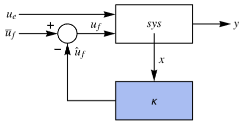
StateFeedbackGains[sys, p, {"ClosedLoopSystem", <|"Merge" -> False|>}]SystemsModelMerge[%]StateFeedbackGains[sys, p, {"ClosedLoopSystem", <|"Merge" -> True|>}]sm = CreateSystemModel["MassSpringDamper", {m x''[t] + c x'[t] + k x[t] == u[t], y[t] == x[t]}, t, {"u"∈"Modelica.Blocks.Interfaces.RealInput", "y"∈"Modelica.Blocks.Interfaces.RealOutput"}, <|"ParameterValues" -> {m -> 10, c -> 10^2, k -> 10^3}|>];csysName = "MassSpringDamperWithStateFeedback";csys = StateFeedbackGains[sm, {-2, -3}, {"ClosedLoopSystem", <|"ModelName" -> csysName|>}]csys["ModelName"]SystemModelSimulate[csysName, {"y"}, 10, <|"Inputs" -> {"u" -> UnitStep}|>]SystemModelPlot[%, All]选项 (6)
Method (6)
"Ackermann" 方法默认用于具有精确值或符号值的系统:
ssm = StateSpaceModel[{{{0, 1}, {-k/m, -c/m}},
  {{c/m}, {-c^2/m^2 +
     k/m}}, {{1, 0}}, {{0}}}, SamplingPeriod -> None,
 SystemsModelLabels -> None];
StateFeedbackGains[ssm, {Subscript[p, 1], Subscript[p, 2]}]StateFeedbackGains[ssm, {Subscript[p, 1], Subscript[p, 2]}, Method -> "Ackermann"] === %ssm = StateSpaceModel[{{{-1.2, 0.2}, {1., -4.1}}, {{2., 0}, {0., 1.}}, {{1., 1.1}}, {{0, 0}}},
SamplingPeriod -> None, SystemsModelLabels -> None];
StateFeedbackGains[ssm, {-1., -2.}]StateFeedbackGains[ssm, {-1., -2.}, Method -> "KNVD"] === %LinearSolve 用于输入至少与状态一样多的不精确系统:
StateFeedbackGains[StateSpaceModel[{{{a}}, {{Subscript[b, 1],
    Subscript[b, 2]}}, {{c}}, {{0, 0}}}, SamplingPeriod -> None,
SystemsModelLabels -> None], {p}, Method -> Automatic]LinearSolve[{{Subscript[b, 1], Subscript[b, 2]}}, {{a - p}}]ssm = StateSpaceModel[{{{-1.2, 0.2}, {1., -4.1}}, {{2., 0}, {0., 1.}}, {{1., 1.1}}, {{0, 0}}},
SamplingPeriod -> None, SystemsModelLabels -> None];
p = {-3 + 2 I, -3 - 2I };StateFeedbackGains[ssm, p] === StateFeedbackGains[ssm, p, Method -> "KNVD"]对于多输入系统,"Ackermann" 方法仅使用一个输入:
ssm = StateSpaceModel[{{{-1.2, 0.2}, {1., -4.1}}, {{2., 0}, {0., 1.}}, {{1., 1.1}}, {{0, 0}}},
 SamplingPeriod -> None, SystemsModelLabels -> None];
p = {-3 + 2 I, -3 - 2I };κ = StateFeedbackGains[ssm, p, Method -> "Ackermann"]Position[κ, {0..}]Table[SingularValueList[ControllabilityMatrix[SystemsModelExtract[ssm, i]]], {i, 2}];Table[i[[1]] / i[[-1]], {i, %}]"KNVD" 闭环极点对反馈增益扰动的敏感度低于 "Ackermann":
ssm = StateSpaceModel[{{{-10, 0, -10, 0}, {0, -0.7, 9, 0}, {0, -1, -0.7, 0}, {1, 0, 0, 0}},
  {{20, 2.8}, {0, -3.13}, {0, 0}, {0, 0}}}, SamplingPeriod -> None, SystemsModelLabels -> None];
p = {-10, -8, -5, -2};MatrixForm /@ {Subscript[κ, 1] = StateFeedbackGains[ssm, p, Method -> "KNVD"], Subscript[κ, 2] = StateFeedbackGains[ssm, p, Method -> "Ackermann"]}δp = RandomReal[{-0.1, 0.1}, Dimensions[Subscript[κ, 1]]];
MatrixForm /@ {Subscript[κ, 1] += δp, Subscript[κ, 2] += δp}csys = Table[SystemsModelStateFeedbackConnect[ssm, κ], {κ, {Subscript[κ, 1], Subscript[κ, 2]}}];
{Subscript[p, 1], Subscript[p, 2]} = Table[Eigenvalues@First@Normal[sys], {sys, csys}]Table[Norm[(pl - p/p), Infinity], {pl, {Subscript[p, 1], Subscript[p, 2]}}]应用 (14)
机械系统 (4)
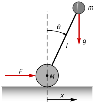
segw = NonlinearStateSpaceModel[IconizedObject[«eqns»] /. IconizedObject[«pars»], {x[t], x'[t], {θ[t], 0}, θ'[t]}, f[t], {x[t], θ[t]}, t]//SimplifyOutputResponse[{segw, {0, 0, 0.1}}, 0, {t, 0, 10}];
Plot[%, {t, 0, 10}, PlotRange -> All, PlotLegends -> {θ, x}]segw = NonlinearStateSpaceModel[segw, Automatic, Automatic, Automatic, None];p = {-2 + 0.5I, -2 - 0.5I, -3.5, -1.5};
𝒸𝒹 = StateFeedbackGains[segw, p, "Data"]𝒸𝒹["ClosedLoopPoles"]𝒸𝒹["OpenLoopPoles"]csys = 𝒸𝒹["ClosedLoopSystem"]//FullSimplifysr = StateResponse[{csys, {0, 0, 0.1}}, 0, {t, 0, 10}];
Table[Plot[𝓈𝓇[[1]], {t, 0, 15}, IconizedObject[«plotOpts»]], {𝓈𝓇, ({sr, {θ, ω, x, x'}})}]or = OutputResponse[csys, 0.2UnitBox[t - 1], {t, 0, 20}];
Table[Plot[ℴ𝓇[[1]], {t, 0, 15}, IconizedObject[«plotOpts»]], {ℴ𝓇, ({or, {θ, x}})}]OutputResponse[𝒸𝒹["ControllerModel"], Join[{0}, sr], {t, 0, 10}];
Plot[%, {t, 0, 10}, PlotRange -> All]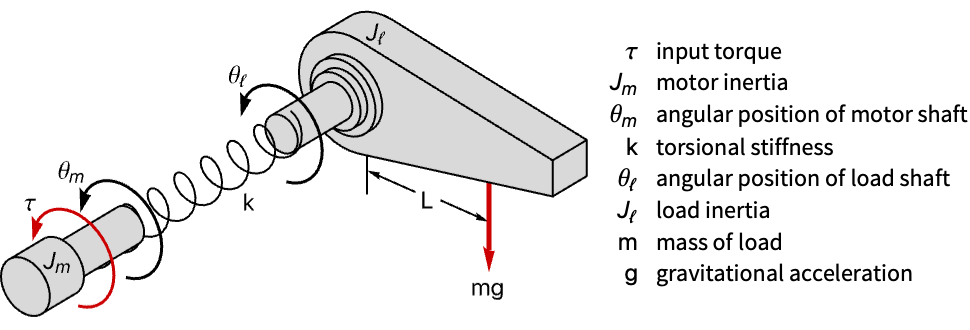
robotM = NonlinearStateSpaceModel[IconizedObject[«eqns»] /. IconizedObject[«pars»], {θ[t], θ'[t], ϕ[t], ϕ'[t]}, τ[t], θ[t], t];
robotM = NonlinearStateSpaceModel[robotM, Automatic, Automatic, Automatic, None]OutputResponse[{robotM, {0.2}}, 0, {t, 0, 15}];
Plot[%, {t, 0, 15}, PlotRange -> All]p = {-1 + I, -1 - I, -4 + 0.25I, -4 - 0.25I};
𝒸𝒹 = StateFeedbackGains[robotM, p, "Data"]csys = 𝒸𝒹["ClosedLoopSystem"]sr = StateResponse[{csys, {0.05}}, 0, {t, 0, 15}];
Table[Plot[𝓈𝓇[[1]], {t, 0, 15}, IconizedObject[«plotOpts»]], {𝓈𝓇, ({sr, {θ, θ', ϕ, ϕ'}})}]cm = 𝒸𝒹["ControllerModel"]OutputResponse[cm, Join[{0}, sr], {t, 0, 10}];
Plot[%, {t, 0, 10}, PlotRange -> All]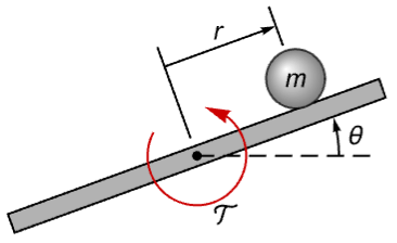
bbs = StateSpaceModel[IconizedObject[«eqns»] /. IconizedObject[«pars»], {r[t], θ[t]}, 𝒯[t], r[t], t, IconizedObject[«labels»]]
τ = 0.2;
bbd = ToDiscreteTimeModel[bbs, τ]OutputResponse[{bbd, {0, 0, 0.01}}, Table[0, 10]];
ListStepPlot[%, DataRange -> {0, 9 τ}, PlotRange -> All]p = {0.7, -0.75, 0.05 + 0.0125I, 0.05 - 0.0125I};
𝒸𝒹 = StateFeedbackGains[bbd, p, "Data"]csys = 𝒸𝒹["ClosedLoopSystem"]sr = StateResponse[{csys, {0, 0, 0.25, 0}}, Table[0, 30]];
ListStepPlot[%[[1]], DataRange -> {0, 29 τ}, PlotRange -> All]OutputResponse[𝒸𝒹["ControllerModel"], Join[{Table[0, 30]}, sr]];
ListStepPlot[%, DataRange -> {0, 29 τ}, PlotRange -> All]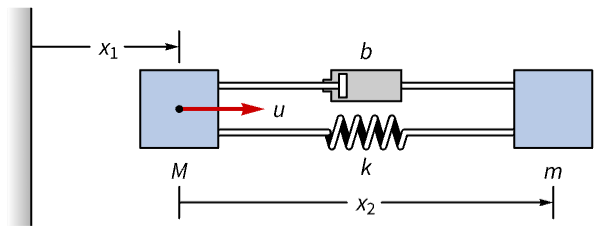
ssm = StateSpaceModel[IconizedObject[«eqns»] /. IconizedObject[«pars»], {Subscript[x, 1][t], Subscript[x, 1]'[t], Subscript[x, 2][t], Subscript[x, 2]'[t]}, u[t], {Subscript[x, 1][t], Subscript[x, 2][t]}, t, IconizedObject[«labels»]]
τ = 0.4;
ssmd = ToDiscreteTimeModel[ssm, 0.4, Method -> "ZeroOrderHold"]

OutputResponse[{ssmd, {1}}, Table[0, 30]];
ListStepPlot[%, DataRange -> {0, 29 τ}, IconizedObject[«plotOpts»]]Subscript[𝒸𝒹, 1] = StateFeedbackGains[ssmd, {0.9, 0.4, 0.3, 0.1}, "Data"]Subscript[𝒸𝒹, 2] = StateFeedbackGains[ssmd, {0.75 + 0.4I, 0.75 - 0.4I, 0.1, 0.2}, "Data"]{Subscript[csys, 1], Subscript[csys, 2]} = Table[Subscript[𝒸𝒹, i]["ClosedLoopSystem"], {i, 2}]{Subscript[sr, 1], Subscript[sr, 2]} = Table[StateResponse[{Subscript[csys, i], {1}}, Table[0, 30]], {i, 2}];Table[ListStepPlot[Subscript[sr, i][[{1, 3}]], DataRange -> {0, 29τ}, IconizedObject[«plotOpts»]], {i, 2}]{Subscript[κ, 1], Subscript[κ, 2]} = Table[Subscript[𝒸𝒹, i]["FeedbackGains"], {i, 2}]Table[ListStepPlot[-Subscript[κ, i].Subscript[sr, i], PlotRange -> All, ImageSize -> Small], {i, 2}]机电系统 (1)
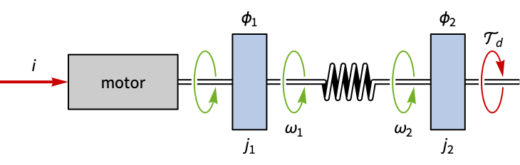
gauge = StateSpaceModel[IconizedObject[«eqns»] /. IconizedObject[«pars»], {Subscript[ϕ, 1][t], Subscript[ω, 1][t], Subscript[ϕ, 2][t], Subscript[ω, 2][t]}, {i[t] , Subscript[𝒯, d][t]}, Subscript[ϕ, 2][t], t, IconizedObject[«labels»]]OutputResponse[{gauge, {0.1, 0, -0.1}}, {0, 0}, {t, 0, 200}];
Plot[%, {t, 0, 200}, PlotRange -> All]sspec = <|"InputModel" -> gauge, "FeedbackInputs" -> 1|>;p = {-2, -1.5, -1 + I, -1 - I};
𝒸𝒹 = StateFeedbackGains[sspec, p, "Data"]𝒸𝒹["ClosedLoopPoles"]csys = 𝒸𝒹["ClosedLoopSystem"]sr = StateResponse[{csys, {0.1, 0, -0.1}}, {0, 0}, {t, 0, 10}];
Plot[%[[4]], {t, 0, 10}, PlotRange -> All]OutputResponse[csys, {0, 0.1Sin[t]}, {t, 0, 100}];
Plot[%, {t, 0, 100}, PlotRange -> {1, -1}]cm = 𝒸𝒹["ControllerModel"]OutputResponse[cm, Join[{0}, sr], {t, 0, 10}];
Plot[%, {t, 0, 10}, IconizedObject[«plotOpts»]]航空航天系统 (2)
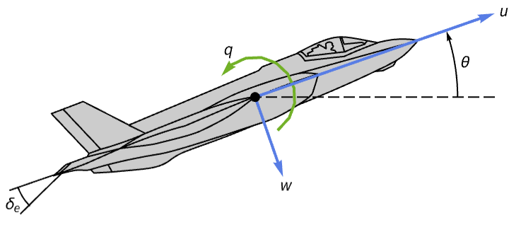
aircraft = NonlinearStateSpaceModel[IconizedObject[«eqns»] /. IconizedObject[«pars»], {u[t], w[t], q[t], θ[t]}, Subscript[δ, e][t], θ[t], t]其俯仰角在受到初始扰动后需要大约 1500 秒才能稳定下来:
OutputResponse[{aircraft, {0, 0, 0, 0.1}}, 0, {t, 0, 2000}];
Plot[%, {t, 0, 2000}, PlotRange -> All]aircraft = NonlinearStateSpaceModel[aircraft, Automatic, Automatic, Automatic, None];p = {-3, -1 + 0.5I, -1 - 0.5I, -1};
𝒸𝒹 = StateFeedbackGains[aircraft, p, "Data"]csys = 𝒸𝒹["ClosedLoopSystem"]sr = StateResponse[{csys, {0, 0, 0.1, 0}}, 0, {t, 0, 15}];
Table[Plot[𝓈𝓇[[1]], {t, 0, 15}, IconizedObject[«plotOpts»]], {𝓈𝓇, ({sr, {u, w, q, θ}})}]cm = 𝒸𝒹["ControllerModel"]OutputResponse[cm, Join[{0}, sr], {t, 0, 20}];Plot[%, {t, 0, 5}, PlotRange -> All]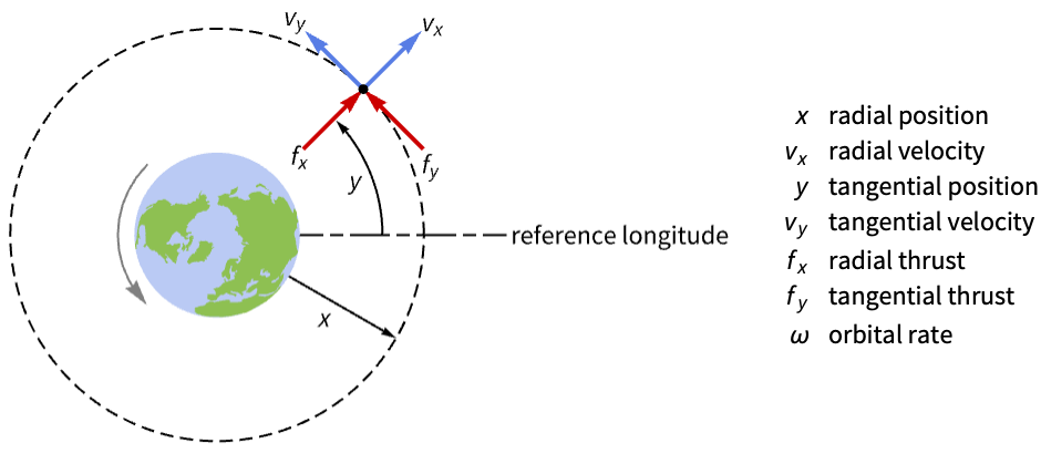
sat = StateSpaceModel[IconizedObject[«eqns»] /. ω -> 0.0011, {x[t], x'[t], y[t], y'[t]}, {Subscript[f, x][t], Subscript[f, y][t]}, {x[t], y[t]}, t, IconizedObject[«labels»]]OutputResponse[{sat, {0, 0.2, 0, 0.1}}, {0, 0}, {t, 0, 10}];
Table[Plot[%[[i]], {t, 0, 10}, IconizedObject[«plotOpts»]], {i, 2}]MatrixForm[κ = StateFeedbackGains[sat, {-0.5, -1.5, -1, -2.5}]]MatrixForm[ℓ = EstimatorGains[sat, 3 {-0.5, -1.5, -1, -2.5}]]ℯ𝓇 = EstimatorRegulator[sat, {ℓ, κ}, "Data"]csys = ℯ𝓇["ClosedLoopSystem"]or = OutputResponse[{csys, {0, 0.2, 0, 0.1}}, {0, 0}, {t, 0, 15}];
Plot[or, {t, 0, 15}, IconizedObject[«plotOpts»]]cm = ℯ𝓇["ControllerModel"]OutputResponse[cm, Join[{0}, or], {t, 0, 15}];
Plot[%, {t, 0, 15}, IconizedObject[«plotOpts»]]电气系统 (3)
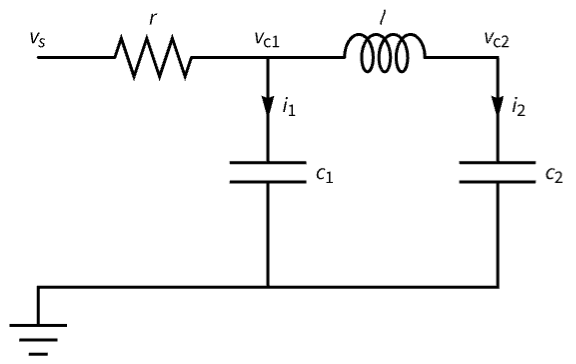
circuit = StateSpaceModel[Join[IconizedObject[«comps»], IconizedObject[«eqns»]], IconizedObject[«vars»], Subscript[v, s][t], Subscript[v, c2][t],
t, DescriptorStateSpace -> True, IconizedObject[«labels»]] /. IconizedObject[«pars»]OutputResponse[circuit, UnitStep[t], {t, 0, 10}];
Plot[%, {t, 0, 10}, PlotRange -> All, ImageSize -> Small]TransferFunctionPoles@TransferFunctionModel[circuit]//Np = {-2, -5 + I, -5 - 1I};
𝒸𝒹 = StateFeedbackGains[circuit, p, "Data"]csys = 𝒸𝒹["ClosedLoopSystem"]sr = StateResponse[csys, UnitStep[t], {t, 0, 10}];
Plot[%[[2]], {t, 0, 10}, PlotRange -> All]BodePlot[{circuit, csys}, IconizedObject[«plotOpts»]]Plot[-𝒸𝒹["FeedbackGains"].sr, {t, 0, 10}, PlotRange -> All]tfm = BiquadraticFilterModel[{"Bandpass", {{60, 5}}}, s]filter = StateSpaceModel[tfm]TransferFunctionPoles[tfm][[1, 1]]//Np = {{-6 + 50I, -6 - 50I}, {-15 + 40I, -15 - 40I}, {-25 + 30I, -25 - 30I}};
csys = Table[StateFeedbackGains[filter, 𝓅, "ClosedLoopSystem"], {𝓅, p}]or = Table[OutputResponse[sys, Sin[t], {t, 0, 2}], {sys, Join[{filter}, csys]}];
Table[Plot[ℴ𝓇[[1]], {t, 0, 2}, IconizedObject[«plotOpts»]], {ℴ𝓇, ({or, IconizedObject[«plotLabels»]})}]dcMot = StateSpaceModel[TransferFunctionModel[{{{100.23330719585297}}, 1 + 0.8*s}, s], SystemsModelLabels -> {"v", "ω"}]sspec = <|"InputModel" -> dcMot, "TrackedOutputs" -> 1|>𝒸𝒹 = StateFeedbackGains[sspec, {-1.5, -2}, "Data"]ℓ = EstimatorGains[sspec, {-3}]ℯ𝓇 = EstimatorRegulator[sspec, {ℓ, 𝒸𝒹}, "Data"]csys = ℯ𝓇["ClosedLoopSystem"]
ref = 200;
or = OutputResponse[csys, ref, {t, 0, 7}];Plot[{or, ref}, {t, 0, 7}, IconizedObject[«plotOpts»]]OutputResponse[ℯ𝓇["ControllerModel"], {ref, or[[1]]}, {t, 0, 5}]
Plot[%, {t, 0, 5}, PlotRange -> All]化学系统 (2)
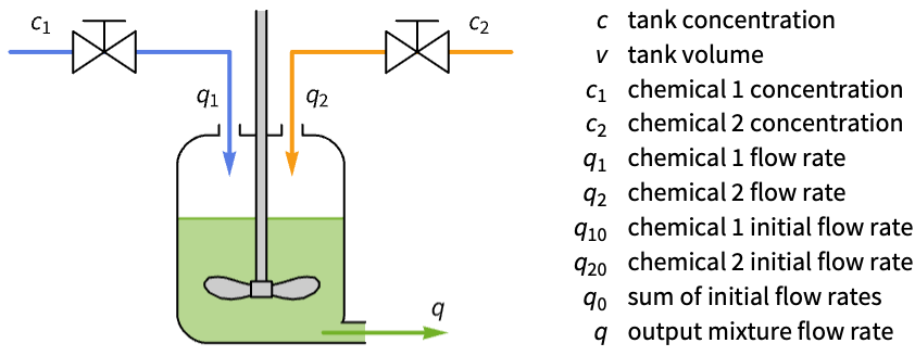
ssm = StateSpaceModel[IconizedObject[«eqns»], IconizedObject[«vars»], IconizedObject[«labels»], DescriptorStateSpace -> True] /. Subscript[q, 0] -> Subscript[q, 10] + Subscript[q, 20] /. IconizedObject[«pars»]olor = OutputResponse[ssm, {0, UnitBox[t - 1]}, {t, 0, 300}];
Plot[olor, {t, 0, 300}, PlotRange -> All]𝒸𝒹 = StateFeedbackGains[ssm, {-0.5, -0.3}, "Data"]csys = 𝒸𝒹["ClosedLoopSystem"]//Chopclsr = StateResponse[csys, {0, UnitBox[t - 5]}, {t, 0, 300}];
Plot[{olor, clsr[[3]]}, {t, 0, 300}, IconizedObject[«plotOpts»]]κ = 𝒸𝒹["FeedbackGains"]Plot[Evaluate[-κ.clsr], {t, 0, 50}, IconizedObject[«plotOpts»]]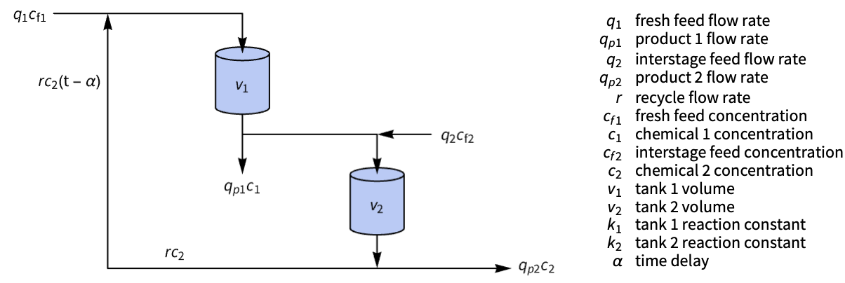
reactor = StateSpaceModel[IconizedObject[«eqns»], {Subscript[c, 1][t], Subscript[c, 2][t]}, {Subscript[c, f1][t], Subscript[c, f2][t]},
{Subscript[c, 1][t - Subscript[τ, 1]], Subscript[c, 2][t - Subscript[τ, 2]]}, t, IconizedObject[«labels»]] /. IconizedObject[«pars»]OutputResponse[{reactor, {0.1, -0.1}}, {0, 0}, {t, 0, 10}];
Plot[%, {t, 0, 10}, IconizedObject[«plotOpts»]]dfsys = MinimalStateSpaceModel[SystemsModelDelayApproximate[reactor, 0]]κ = StateFeedbackGains[dfsys, {-3 + I, -3 - I}]ℓ = EstimatorGains[dfsys, {-5, -6}]ℯ𝓇 = EstimatorRegulator[dfsys, {ℓ, κ}, "EstimatorRegulatorFeedbackModel"]smC = SmithDelayCompensator[reactor, ℯ𝓇]csys = SystemsModelFeedbackConnect[SystemsModelSeriesConnect[smC, reactor]]OutputResponse[{csys, {0.1, -0.1}}, {0, 0}, {t, 0, 10}];
Plot[%, {t, 0, 10}, IconizedObject[«plotOpts»]]无差拍控制 (1)
dssm = StateSpaceModel[{{{1, 1, -2}, {0, 1, 1}, {0, 0, 1}}, {{1}, {0}, {1}}}, SamplingPeriod -> 1,
SystemsModelLabels -> None];csys = StateFeedbackGains[dssm, {0, 0, 0}, "ClosedLoopSystem"]
SystemsModelOrder[dssm]or = OutputResponse[{csys, RandomReal[{-1, 1}, 3]}, Table[0, 6]]//ChopListStepPlot[or, Right, PlotRange -> All, DataRange -> {0, 5}]航海系统 (1)
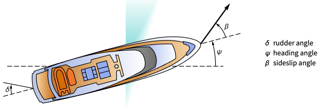
boat = StateSpaceModel[IconizedObject[«abc»], IconizedObject[«labels»]]sspec = <|"InputModel" -> boat, "TrackedOutputs" -> 1|>;cd = StateFeedbackGains[sspec, {-0.35, -0.3, -0.25 + 0.1I, -0.25 - 0.1I}, "Data"]csys = cd["ClosedLoopSystem"]Table[OutputResponse[csys, ref, {t, 0, 50}], {ref, 4, 20, 4}];
Plot[%, {t, 0, 50}, IconizedObject[«plotOpts»]]cm = cd["ControllerModel"]cinps[ref_] := Join[{ref}, OutputResponse[csys, ref, {t, 0, 50}], StateResponse[csys, ref, {t, 0, 50}][[1 ;; 3]]]Table[OutputResponse[cm, cinps[ref], {t, 0, 50}], {ref, 4, 20, 4}];
Plot[%, {t, 0, 50}, IconizedObject[«plotOpts»]]属性和关系 (17)
a = RandomReal[{-1, 1}, {2, 2}];
b = RandomReal[{-1, 1}, {2, 1}];
p = RandomReal[{-3, -1}, 2];κ = StateFeedbackGains[StateSpaceModel[{a, b}], p]p1 = Eigenvalues[a - b.κ]ContainsExactly[p1, p, SameTest -> (Chop[#1 - #2] == 0. &)]𝒸𝒹 = StateFeedbackGains[StateSpaceModel[{{{-1, 2}, {1, 3}}, {{1}, {0}}, {{1, 0}}, {{0}}}, SamplingPeriod -> None,
SystemsModelLabels -> None], {-3, -4}, "Data"]SystemsModelStateFeedbackConnect[𝒸𝒹["InputModel"], 𝒸𝒹["FeedbackGains"]]𝒸𝒹["ClosedLoopSystem"]ssm = StateSpaceModel[{{{-3, 0}, {0, -2}}, {{1}, {-1}}}, SamplingPeriod -> None,
SystemsModelLabels -> None];
p = {{-3, -2}, {-3, -2.5}, {-2.5, -2}, {-4, -1}, {-4, -5}};ListLinePlot[Table[{Norm[𝓅 - {-3, -2}], Norm@StateFeedbackGains[ssm, 𝓅]}, {𝓅, p}], IconizedObject[«plotOpts»]]
nsys = NonlinearStateSpaceModel[{{-2*Subscript[x, 1] + Subscript[x, 1]^2 +
    Subscript[x, 2], 1 + u - Subscript[x, 1] -
    Subscript[x, 2] + Subscript[x, 1]*Subscript[x, 2]},
  {Subscript[x, 1]}}, {{Subscript[x, 1], 1},
  {Subscript[x, 2], 1}}, {u}, {Automatic}, Automatic,
 SamplingPeriod -> None];
p = {-4 + I, -4 - I};StateFeedbackGains[nsys, p]
κ = StateFeedbackGains[StateSpaceModel[nsys], p]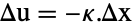
-SolveValues[{u - 1} == -κ.{Subscript[x, 1] - 1, Subscript[x, 2] - 1}, u]可控标准 StateSpaceModel 的所有极点都可以使用状态反馈来控制:
ssm = StateSpaceModel[{{{0, 1}, {-1, -2}}, {{0}, {1}}, {{1, 0}}, {{0}}}, SamplingPeriod -> None,
SystemsModelLabels -> None];ControllableModelQ[ssm]p = Eigenvalues[Normal[ssm][[1]]] - RandomReal[{1, 3}, 2]cd = StateFeedbackGains[ssm, p, "Data"];
cd["FeedbackGains"]ContainsExactly[cd["ClosedLoopPoles"], p, SameTest -> (Chop[#1 - #2] == 0.&)]可控的非奇异描述符 StateSpaceModel 的所有极点也可以被控制:
dssm = StateSpaceModel[{{{1, 1}, {0, 0}}, {{0}, {1}}, {{3, 8}}, {{0}}, {{1, 0}, {1, 1}}},
SamplingPeriod -> None, SystemsModelLabels -> None];{ControllableModelQ[dssm], MatrixRank[Last[Normal[dssm]]]}p = Eigenvalues[Normal[dssm][[{1, -1}]]] - RandomReal[{1, 3}, 2]𝒸𝒹 = StateFeedbackGains[dssm, p, "Data"]𝒸𝒹["FeedbackGains"]ContainsExactly[𝒸𝒹["ClosedLoopPoles"], p, SameTest -> (Chop[#1 - #2] == 0.&)]只能控制不可控的标准 StateSpaceModel 的子系统:
ssm = StateSpaceModel[{{{-2., 0}, {0, -1}}, {{1}, {0}}, {{1, 1}}, {{0}}}, SamplingPeriod -> None,
 SystemsModelLabels -> None];

modes = Eigenvalues[First[Normal[ssm]]];
Table[{λ, ControllableModelQ[{ssm, {λ}}]}, {λ, modes}]

𝒸𝒹 = StateFeedbackGains[ssm, {-RandomReal[{4, 8}], -1}, "ClosedLoopPoles"]StateFeedbackGains[ssm, {-RandomReal[{4, 8}], -RandomReal[{4, 8}]}, "ClosedLoopPoles"]
dssm = StateSpaceModel[{{{-5, 0}, {0, 1}}, {{1}, {0}}, {{1, 0}}, {{0}}, {{1, 0}, {0, 0}}},
 SamplingPeriod -> None, SystemsModelLabels -> None];
ControllableModelQ[{dssm, "Slow"}]dim = Total[Diagonal[Normal[dssm][[5]]]]p = RandomReal[{-8, -6}, dim]
𝒸𝒹 = StateFeedbackGains[dssm, p, "Data"];
𝒸𝒹["FeedbackGains"]
慢子系统的极点移动到所需位置,快子系统对应的  处的极点不变:
{𝒸𝒹["OpenLoopPoles"], 𝒸𝒹["ClosedLoopPoles"]}{ControllableModelQ[dssm], SystemsModelOrder[dssm]}dssm = StateSpaceModel[{{{-5, 0}, {0, 1}}, {{0}, {0}}, {{1, 0}}, {{0}}, {{1, 0}, {0, 0}}},
SamplingPeriod -> None, SystemsModelLabels -> None];
ControllableModelQ[{dssm, "Slow"}]dim = Total[Diagonal[Normal[dssm][[5]]]]p = RandomReal[{-8, -6}, dim]StateFeedbackGains[dssm, p, {"OpenLoopPoles", "ClosedLoopPoles"}]
LQRegulatorGains 和 StateFeedbackGains 对单输入系统产生相同的结果:
ssm = StateSpaceModel[{{{0, 1}, {-2, -0.5}}, {{0}, {1}}, {{1, 0}}, {{0}}}, SamplingPeriod -> None,
 SystemsModelLabels -> None];
𝒸𝒹 = LQRegulatorGains[ssm, {(|   |   |
| - | - |
| 2 | 0 |
| 0 | 1 |), (1)}, "Data"];
StateFeedbackGains 与 LQRegulatorGains 设计的闭环极点:
StateFeedbackGains[ssm, 𝒸𝒹["ClosedLoopPoles"]]LQRegulatorGains 给出相同增益:
𝒸𝒹["FeedbackGains"]可以使用对称根轨迹图获得最小化  ρ c.c x(t)2+u(t)2t 的闭环极点:
ssm = StateSpaceModel[{{{-2, 0, 0}, {1, 0, 0}, {0, 1, 0}}, {{1}, {0}, {0}}, {{0, 0, 1}}, {{0}}},
SamplingPeriod -> None, SystemsModelLabels -> {u, y}];symTFM = With[{tfm = TransferFunctionModel[ssm, s]}, tfm[s] tfm[-s]][[1, 1]];
symRLPlot = RootLocusPlot[ρ symTFM, {ρ, 0, 20}]
p = Cases[symRLPlot, Tooltip[{___, Point[{{x_ ? Negative, y_}}]}, ρ == 10.] :> x + I y, {0, Infinity}]StateFeedbackGains[ssm, p, "FeedbackGains"]使用 LQRegulatorGains 会获得相同增益:
c = Normal[ssm][[3]];
LQRegulatorGains[ssm, {10 c.c, {{1.}}}, "FeedbackGains"]对于 StateSpaceModel 而言,StateFeedbackGains 和 FullInformationOutputRegulator 给出相同结果:
ssm = StateSpaceModel[{{{2, 0, -1}, {0, -2, 1}, {1, -1, 1}}, {{1, 1}, {0, 1}, {1, -1}},
{{1, -1, 0}, {0, 1, -1}}, {{0, 0}, {0, 0}}}, SamplingPeriod -> None, SystemsModelLabels -> None];p = {-1, -2, -3};StateFeedbackGains[ssm, p] === FullInformationOutputRegulator[ssm, p]ssm = StateSpaceModel[{{{0, 1, 0}, {0, 0, -1}, {0, 0, 0.5}}, {{0}, {1}, {1}}, {{1, 2, 4}}, {{0}}},
SamplingPeriod -> 1, SystemsModelLabels -> None];{ℓ, κ} = {EstimatorGains[ssm, {-1, -1 + I, -1 - I}], StateFeedbackGains[ssm, {-1, -1 + I, -1 - I}]}er = EstimatorRegulator[ssm, {ℓ, κ}]
κ = RandomReal[{0, 10}];
tfm = TransferFunctionModel[{{{k}}, (1 + s)*(2 + s)*
(3 + s)}, s];Subscript[p, cl] = TransferFunctionPoles[SystemsModelFeedbackConnect[tfm /. k -> κ]][[1, 1]]ssm = StateSpaceModel[tfm, StateSpaceRealization -> "ControllableCompanion"]对于这种实现,状态反馈增益的形式为 {{κ,0,…,0}}:
Chop[StateFeedbackGains[ssm, Subscript[p, cl]]] == {{κ, 0, 0}}κ = RandomReal[{0, 10}];
tfm = TransferFunctionModel[{{{k}}, (1 + s)*(2 + s)*
(3 + s)}, s];Subscript[p, cl] = TransferFunctionPoles[SystemsModelFeedbackConnect[tfm /. k -> κ]][[1, 1]]ssm = StateSpaceModel[tfm, StateSpaceRealization -> "ControllableCompanion"]对于这种实现,状态反馈增益的形式为 {{κ,0,…,0}}:
Chop[StateFeedbackGains[ssm, Subscript[p, cl]]] == {{κ, 0, 0}}{ssm = StateSpaceModel[{{{0, 1, 0, 0}, {0, 0, -1, 0}, {0, 0, 0, 1}, {0, 0, 11, 0}}, {{0}, {1}, {0}, {1}},
{{1, 2, 3, 4}}, {{0}}}, SamplingPeriod -> None, SystemsModelLabels -> None], dualssm = DualSystemsModel[ssm]}p = {-1, -2, -1 + I, -1 - I};
κ = StateFeedbackGains[ssm, p]ℓ = EstimatorGains[dualssm, p]{κ == ℓ, ℓ == κ}ssm = StateSpaceModel[{{{0, 1, 0}, {0, 0, 1}, {-1, -2, -2}}, {{0}, {0}, {1}}, {{4, 0, 1}}, {{0}}},
SamplingPeriod -> None, SystemsModelLabels -> None];TransferFunctionZeros[TransferFunctionModel[ssm]]csys = StateFeedbackGains[ssm, {-3 + 2 I, -3 - 2 I, -7}, "ClosedLoopSystem"]开环和闭环系统都阻塞输入 Sin[2t]:
or = Table[OutputResponse[sys, Sin[2t], t], {sys, {ssm, csys}}];
{Plot[or[[1]], {t, 0, 15}, IconizedObject[«plotOpts»]], Plot[or[[2]], {t, 0, 3}, IconizedObject[«plotOpts»]]}ssm = StateSpaceModel[{{{0, 1}, {-12, -8.}}, {{0}, {1}}, {{4, 1}}, {{0}}}, SamplingPeriod -> None,
SystemsModelLabels -> None];z = TransferFunctionZeros[TransferFunctionModel[ssm]]//Flattenp = {z[[1]], -8};
csys = StateFeedbackGains[ssm, p, "ClosedLoopSystem"]ObservableModelQ[csys]可能存在的问题 (5)
ssm = StateSpaceModel[{{{-1, 0}, {0, -3}}, {{1}, {0}}, {{1, 2}}, {{0}}}, SamplingPeriod -> None,
 SystemsModelLabels -> None];
ControllableModelQ[ssm]StateFeedbackGains[ssm, {-4, -5}]
dssm = StateSpaceModel[{{{-5, 0}, {0, 1}}, {{0}, {0}}, {{1, 0}}, {{0}}, {{1, 0}, {0, 0}}},
 SamplingPeriod -> None, SystemsModelLabels -> None];
{ControllableModelQ[dssm], ControllableModelQ[{dssm, "Slow"}]}dim = Total[Diagonal[Normal[dssm][[5]]]]StateFeedbackGains[dssm, RandomReal[{-8, -6}, dim], {"OpenLoopPoles", "ClosedLoopPoles"}]
StateFeedbackGains[StateSpaceModel[{{{-3, 0}, {0, 2}}, {{1}, {0}}}, SamplingPeriod -> None, SystemsModelLabels -> None], RandomInteger[{-10, -1}, 2]]
ssm = StateSpaceModel[{{{-1, 0, 1}, {-3, 1, 2}, {1, -1, 2}}, {{1, 0}, {0, 1}, {1, -2}}},
SamplingPeriod -> None, SystemsModelLabels -> None];p = {-5 + I, -5 - I, -6};
κ = StateFeedbackGains[ssm, p, Method -> "KNVD"]
StateFeedbackGains[ssm//N, p, Method -> "KNVD"]StateFeedbackGains[ssm, p, Method -> "Ackermann"]ssm = StateSpaceModel[{{{0, 2, 0, 0, -2, 0}, {1, 0, 0, 0, 0, -1}, {0, 1, 0, 0, 0, 0}, {0, 0, 0, 3, 0, 0},
{2, 0, 0, 1, 0, 0}, {0, 0, -1, 0, 1, 0}}, {{1, 2}, {0, 0}, {0, 1}, {0, -1}, {0, 1}, {0, 0}}},
SamplingPeriod -> None, SystemsModelLabels -> None];
p = {-1, -2, -3, -4, -5, -7};{$SystemID, Subscript[κ, 1] = StateFeedbackGains[ssm//N, p, Method -> "KNVD"]}{$SystemID, Subscript[κ, 2] = StateFeedbackGains[ssm//N, p, Method -> "KNVD"]}{$SystemID, With[{ssN = Normal[ssm]}, Eigenvalues[ssN[[1]] - ssN[[2]].Subscript[κ, 1]]]}{$SystemID, With[{ssN = Normal[ssm]}, Eigenvalues[ssN[[1]] - ssN[[2]].Subscript[κ, 2]]]}文本
Wolfram Research (2010),StateFeedbackGains,Wolfram 语言函数,https://reference.wolfram.com/language/ref/StateFeedbackGains.html (更新于 2021 年).
CMS
Wolfram 语言. 2010. "StateFeedbackGains." Wolfram 语言与系统参考资料中心. Wolfram Research. 最新版本 2021. https://reference.wolfram.com/language/ref/StateFeedbackGains.html.
APA
Wolfram 语言. (2010). StateFeedbackGains. Wolfram 语言与系统参考资料中心. 追溯自 https://reference.wolfram.com/language/ref/StateFeedbackGains.html 年