StateSpaceModel
StateSpaceModel[{a,b,c,d}]
represents the standard state-space model with state matrix a, input matrix b, output matrix c, and transmission matrix d.
StateSpaceModel[{a,b,c,d,e}]
represents a descriptor state-space model with descriptor matrix e.
StateSpaceModel[sys]
gives a state-space model corresponding to the systems model sys.
StateSpaceModel[eqns,{{x1,x10},…},{{u1,u10},…},{g1,…},τ]
gives the state-space model obtained by Taylor linearization about the point (xi0,ui0) of the differential or difference equations eqns with outputs gi and independent variable τ.
Details and Options
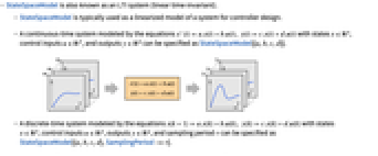
- StateSpaceModel is also known as an LTI system (linear time-invariant).
- StateSpaceModel is typically used as a linearized model of a system for controller design.
- A continuous-time system modeled by the equations
 with states
  , control inputs
  , and outputs
  can be specified as StateSpaceModel[{a,b,c,d}].
 - A discrete-time system modeled by the equations
 with states
  , control inputs
  , outputs
  , and sampling period τ can be specified as StateSpaceModel[{a,b,c,d},SamplingPeriod->τ].
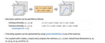
 - Descriptor systems can be specified as follows:
-
StateSpaceModel[{a,b,c,d,e}] 
StateSpaceModel[{a,b,c,d,e},SamplingPeriod->τ] 
- Time delay systems can be represented by using SystemsModelDelay in any of the matrices.
- For a system with n states, p inputs and q outputs, the matrices a, b, c, d and e should have dimensions {n,n}, {n,p}, {q,n}, {q,p} and {n,n}.
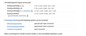
- The following short inputs can be used:
-
StateSpaceModel[{a,b,c}] 
StateSpaceModel[{a,b}] 
StateSpaceModel[{a,b,c,Automatic,e}] =a.x(t)+b.u(t), y(t)=c.x(t)")
StateSpaceModel[{a,b,Automatic,Automatic,e}] =a.x(t)+b.u(t), y(t)=x(t)")
- In StateSpaceModel[sys] the following systems can be converted:
-
AffineStateSpaceModel approximate Taylor conversion NonlinearStateSpaceModel approximate Taylor conversion TransferFunctionModel exact conversion - When converting from transfer-function model sys, the controllable realization is used.
- For equational input, default linearization points xi0 and uj0 are taken to be zero.
- The following options can be given:
-
DescriptorStateSpace Automatic standard or descriptor realization ExternalTypeSignature Automatic variable types for embedded code SamplingPeriod Automatic the sampling period StateSpaceRealization Automatic the canonical realization SystemsModelLabels Automatic the labels for the input, output, and state variables
Examples
open allclose allBasic Examples (4)
Construct a state-space model from state, input, output and transmission matrices:
Construct a state-space model from a transfer function model:
Test its controllability and observability:
Construct a state-space model from a set of ordinary differential equations (ODEs):
Its response to nonzero initial conditions:
Construct a discrete-time state-space model by specifying its sampling period:
Scope (41)
Basic Uses (12)
A state-space model with a state, input, output and transmission matrices:
Its response to a unit-step input:
A state-space model specified using only state, input and output matrices:
The transmission matrix is assumed to be a zero matrix:
A state-space model specified using only state and input matrices:
The states are assumed to be the outputs:
Both models have the same output response:
A discrete-time model with a sampling period of 0.1:
Test its controllability and observability:
A model with 3 states, 2 inputs and 1 output:
Count the number of inputs and outputs:
A model with 3 states, 1 input and 2 outputs:
A multiple-input multiple-output (MIMO) model:
Compute the analytical unit-step response:
They are visible in the AffineStateSpaceModel representation:
If no state variables are specified, they are chosen automatically:
Specify the state, input and output variables:
The NonlinearStateSpaceModel representation:
Use a state-space model to design a pole-placement controller:
The controller design that places the poles at ![]() :
:
The open- and closed-loop poles:
Plot the response of the closed-loop system to a set of initial conditions:
Descriptor Models (6)
Descriptor models are used to model algebraic equations:
It modeled the equation ![]() , where
, where ![]() is the input signal and
is the input signal and ![]() is the output:
is the output:
By default, the descriptor matrix e is assumed to be the identity matrix:
It is equivalent to the following model with an identity descriptor matrix:
Both models have the same state response:
Use Automatic to create a descriptor system with all the states as outputs:
Its state and output responses are the same:
It may be possible to convert a descriptor model to a standard model:
A model with a singular descriptor matrix:
It is still possible to convert it to a standard system:
It may not be possible to convert a descriptor model to a standard one in all cases:
Time-Delay Models (3)
Use SystemsModelDelay to model a system with delays:
It has a delayed output response:
A system with two input delays:
Model Conversions (13)
A state-space model of a transfer-function model:
The state-space representation is not unique:
Both yield same original transfer-function model:
A state-space model of a discrete-time transfer-function model:
A state-space model of an improper transfer-function model yields a descriptor system:
A state-space model of an affine state-space model discards all nonlinearities:
The original model cannot be fully recovered from the linearized model:
If the affine state-space model is linear, no information is lost:
And the original model can be fully recovered:
A state-space model of a nonlinear state-space model discards all nonlinearities:
The original model cannot be fully recovered from the linearized model:
Their output responses are not the same:
If the nonlinear state-space model is linear, no information is lost:
And the original model can be fully recovered:
A state-space model of a system of ODEs:
If the ODEs have nonlinear terms they are approximated:
The nonlinear representation does not approximate the nonlinear terms:
A state-space model of a set of difference equations:
A state-space model of a set of differential-algebraic equations:
Prevent elimination of the algebraic equation:
A state-space model of a set of difference-algebraic equations:
Random Processes (6)
The state-space representation of a MAProcess:
An ARProcess:
An ARMAProcess:
An ARIMAProcess:
A SARMAProcess:
Options (15)
By default, the appearance is selected to fit the display in the notebook:
DescriptorStateSpace (3)
SamplingPeriod (3)
StateSpaceRealization (4)
By default, the controllable companion realization is computed:
Explicitly compute the controllable companion realization:
The observable companion realization:
It is the dual of the controllable companion realization:
The controllable and controllable companion realizations for a MIMO transfer-function model:
The observable and observable companion realizations for a MIMO transfer-function model:
They have a dual relationship with the controllable and controllable companion realizations:
Applications (27)
Mechanical Systems (11)
Compute a state-space model of a mass-spring damper system using Newton's second law:
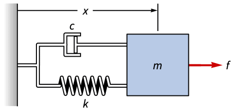
Assemble the equation of the system using ![]() :
:
It is linear and can be put into a linear state-space form without any approximations:
The response of the model to a unit-step input:
Compute a state-space model of an inverted pendulum using the Lagrangian:
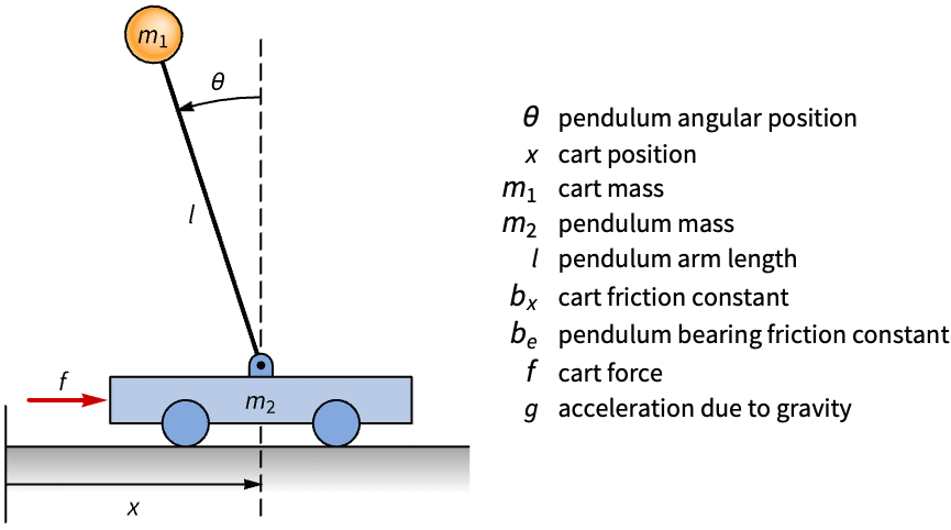
The kinetic energy of the cart and pendulum:
The potential energy of the pendulum:
The nonpositive eigenvalues make it an unstable system:
Compute the state-space model of a vibration absorber using the Lagrangian and the Rayleigh dissipation function:
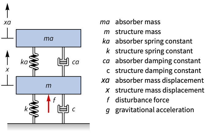
The kinetic energy of the system:
The Rayleigh dissipation function:
The system's equations of motion:
A state-space model of the system:
Its response to an oscillatory disturbance:
Compute the state-space model of a multidomain system consisting of a motor with a load on a flexible shaft:
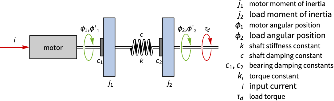
The state response of a numerical model to an input torque from the motor:
Compute an approximate discrete-time state-space model of a ball and beam system starting from continuous-time equations:
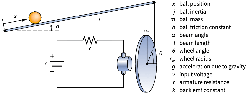
The kinetic energy of the rolling ball, assuming no slipping:
Its potential energy, assuming small tilt-angles of the beam:
The Kirchhoff voltage equation of the tilt-motor, assuming no armature inductance:
The tilt-motor's equation of motion:
The ball and beam's equations:
Construct a numerical state-space model of the ball and beam:
Discretize the model with a sampling period of 50 ![]() :
:
The displacement ![]() of the ball due to a nudge while keeping the beam level:
of the ball due to a nudge while keeping the beam level:
The displacement computed using the discrete-time model:
In both models, the ball will stop rolling due to friction:
An input voltage that tilts the beam back and forth once:
The displacement ![]() of the ball due to the tilts:
of the ball due to the tilts:
The displacement computed using the discrete-time model:
In both models, the ball ends up balanced on a level beam:
Compute state-space models of a pendulum about various equilibrium positions and compare them:
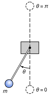
The sinusoidal term makes the model nonlinear:
The equilibrium positions of the pendulum are vertically downward and upward:
A state-space model of the pendulum linearized around a generic equilibrium value ![]() :
:
The state-space models around the two equilibrium positions for a set of parameter values:
The response of the model linearized around 0 is stable, while the one around 180° is unstable:
This is because the two equilibrium points have stable and unstable eigenvalues:
Compute the state-space model of a Wilberforce pendulum that has coupled dynamics and compare the efficacy of different inputs on the pendulum:
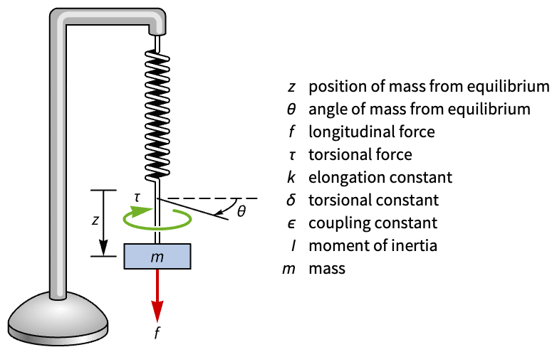
A set of numerical values for the parameters:
Construct a state-space model of the system:
Its output response reveals the coupled dynamics between ![]() and
and ![]() :
:
The system is independently controllable with either the force ![]() or torque
or torque ![]() :
:
A system specification where ![]() is the sole feedback input:
is the sole feedback input:
And one where the torque ![]() is the sole feedback input:
is the sole feedback input:
A pole placement controller to damp the oscillations for each system:
Obtain the closed-loop systems:
The longitudinal oscillations ![]() are damped more effectively by the torque
are damped more effectively by the torque ![]() :
:
The rotational oscillations are damped more effectively by the force ![]() :
:
Obtain the feedback gains of each model:
It takes less effort to dampen the oscillations using ![]() :
:
This can also be seen by quantifying the control effort:
Compute the state-space model of a lathe's cutting process. The delays in the model are necessary to capture the chattering behavior of the system:
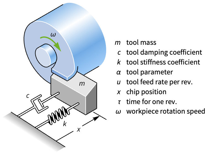
A model of the lathe's cutting process:
The chattering can be seen in the delay model:
Obtain a delay-free approximation:
But the delay-free model does not capture the same chattering:
State-space models allow for state-feedback control techniques like pole placement. Place the poles of the inverted pendulum on the left-hand side of the ![]() -plane to balance the pendulum: »
-plane to balance the pendulum: »
A controller that balances the pendulum using a set of closed-loop poles:
The closed-loop system balances the pendulum when the cart is disturbed:
State-space models are the basis for computing optimal state feedback gains that minimize a cost function. Dampen the oscillations of a flexible shaft using optimal control: »
Set the input current ![]() as the sole feedback input:
as the sole feedback input:
A set of state and control weight matrices ![]() and
and ![]() :
:
Compute the optimal controller that minimizes the cost function ![]() :
:
The oscillations are damped by the controller:
State-space models are also used to solve tracking problems. Design a controller that tracks the position of a ball on a beam: »
Set the system specification to track the ball's position:
A set of state and control weight matrices ![]() and
and ![]() :
:
Compute the tracking controller:
Obtain the closed-loop system:
The closed-loop system places the ball in the middle of the beam:
Aerospace Systems (6)
State-space model are useful in modeling aerospace systems. Construct a state-space model of a satellite's attitude dynamics starting from Euler's equations of motion:

Euler's equations with principal moments of inertia ![]() ,
, ![]() ,
, ![]() :
:
The operating point is an equilibrium point:
Construct a state-space model:
The satellite's attitude is unregulated if disturbed:
Verify the controllability of the model:
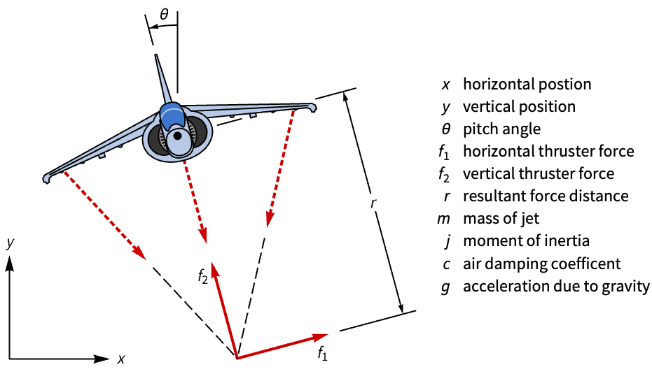
State-space models are used in model analysis. Construct a state-space model of a Harrier VTOL jet and assess its controllability:

Both inputs are needed for the aircraft to be fully controllable:
State-space models are useful for the analysis of MIMO systems where multiple inputs affect a given output. Use the state-space model representation to compare the effectiveness of the aileron and the rudder on the yaw dynamics of a Boeing 747 using state feedback control:
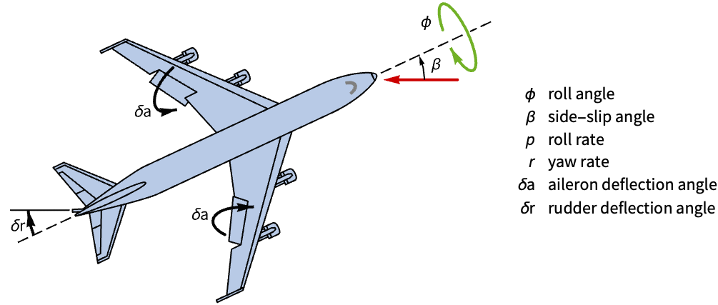
A state-space model of the aircraft's lateral motion from a set of state, input and output matrices:
Obtain a state-space model with the rudder and another with aileron as the sole input:
The closed-loop systems of both systems with an LQR controller:
Using the rudder results in a faster yaw response:
As well as a smaller roll angle:
State-space models are useful for the design of discrete-time state feedback controllers. Obtain a state-space model of the 747's longitudinal dynamics and improve its handling qualities using discrete-time state-feedback control:
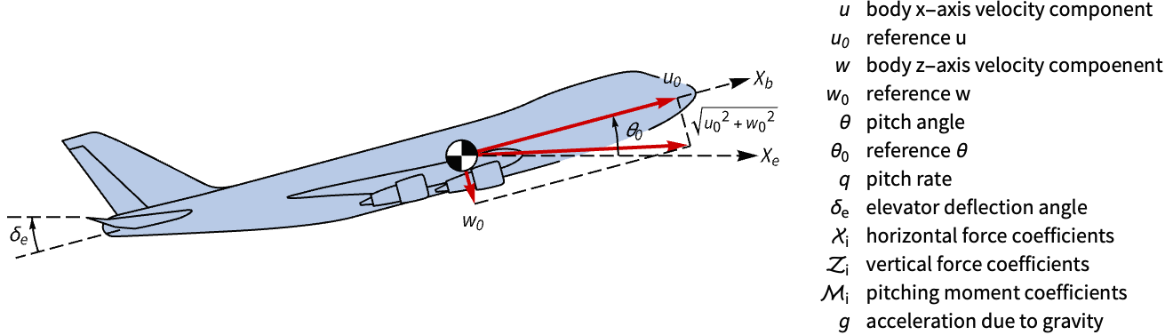
A nonlinear model of the aircraft's longitudinal dynamics:
A linearized state-space model:
Its response to an initial perturbation in the pitch angle ![]() is sluggish and oscillatory:
is sluggish and oscillatory:
This is because the eigenvalues of the linear system are close to the imaginary axis:
A set control weights and sampling period:
Compute the optimal controller that minimizes an approximated discrete-time cost function:
The discrete-time closed-loop system:
The handling qualities are improved:
Discrete-time controllers can also be designed by approximating the continuous-time models. Design a discrete-time controller to stabilize a Harrier VTOL jet by approximating its continuous-time state-space model: »
A state-space model of the Harrier's horizontal dynamics:
Discretize the model with a sampling period of ![]() :
:
Without a controller, the jet's horizontal position is unregulated if its pitch is disturbed:
Design a discrete-time state feedback controller to stabilize the jet:
The discrete-time controller model:
The jet is stabilized with respect to an initial disturbance by the controller:
State-space models can also be used for the design of output feedback controllers such as the estimator regulator. Design an estimator regulator that tracks the angular rate required for a satellite to maintain its nadir-pointing orientation using a discrete-time model: »
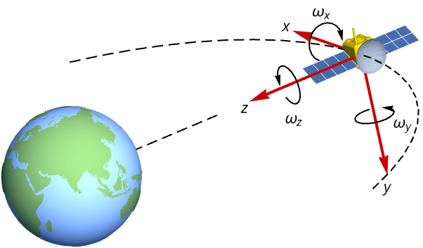
Discretize the model with a sampling period of 0.3:
The radius and gravitational constant mass product of the Earth:
The semimajor axis of the satellite's circular orbit for an altitude of 470 km:
The orbital period is around 94 minutes:
The angular rate is the number of degrees over the orbital period:
Set the system specification to track the satellite's angular rate in the ![]() direction:
direction:
Compute a set of estimator gains:
And a state-feedback controller:
Assemble the estimator regulator:
The satellite now tracks the required angular rate to keep its nadir-pointing orientation:
Biological Systems (2)
Symbolic state-space models can be used to simulate models with parameters. Construct a state-space model of the metabolism of a drug and simulate it:
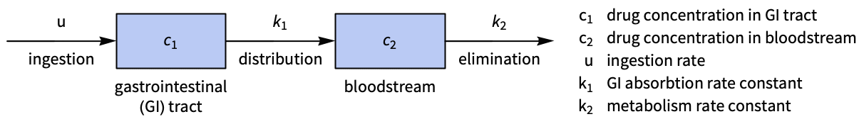
A model the drug's concentrations ![]() and
and ![]() in the GI tract and bloodstream:
in the GI tract and bloodstream:
The analytical expression of its output response to a constant ingestion rate:
Plot the response for different values for the constants ![]() and
and ![]() :
:
State-space models can be used in the design of observers. Starting from an HIV infection model, design an estimator to estimate the free virus population:
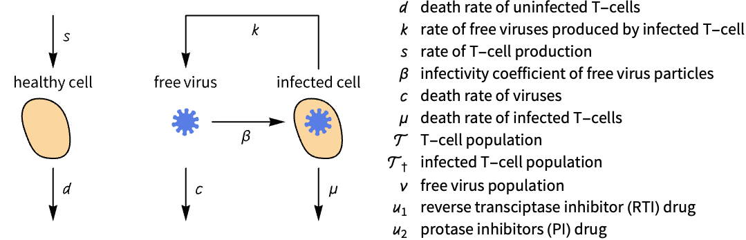
Its equilibrium points and parameter values:
Compare the nonlinear model's free virus population to the estimated virus population:
Chemical Systems (3)
State-space models are useful for modeling chemical reaction processes. Construct a state-space model of a fermentation process and simulate its response to an exponential decay in the dilution rate:
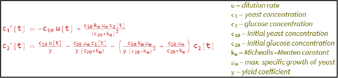
A model of the fermentation process:
An exponential decay in the dilution rate ![]() leads to the halting of the fermentation process:
leads to the halting of the fermentation process:
State-space models are ideal for modeling the chemical dynamics of a continuously stirred-tank reactor (CSTR). Construct a state-space model for the polymerization of methyl-methacrylate (MMA):
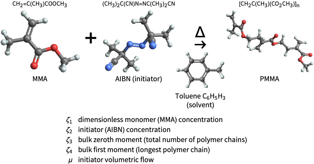
Its poles are on the left side of the ![]() plane, indicating the model is stable:
plane, indicating the model is stable:
The MMA concentration decreases due to an increase in the initiator volumetric flow, indicating PMMA synthesis:
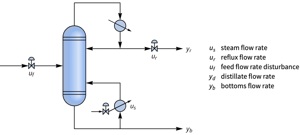
State-space models can be used to model systems with delays. Obtain a state-space model for a distillation column from its Wood–Berry transfer function model and compare its response to a delay-free approximation of the same model:
The Wood–Berry transfer function model of the distillation column:
Its response to a step-input disturbance to the feed is delayed:
Obtain a delay-free approximation of the model:
The delay and delay-free system's responses to a disturbance in the feed input:
Electrical Systems (4)
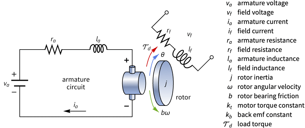
Construct a state-space model of a DC motor with armature and field voltage inputs and analyze its controllability:
The field voltage ![]() is necessary to control the motor:
is necessary to control the motor:
Symbolic state-space models can be used to simulate models with parameters. Construct a symbolic state-space model of an operational amplifier (op amp) circuit from its governing equations and analyze its output phase and amplitude with different parameter values:
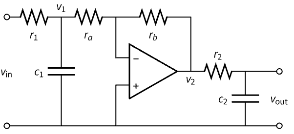
The governing equations using Kirchhoff's current law (KCL):
Obtain two state-space models with different values for ![]() and
and ![]() :
:
The first set of capacitance values attenuates the input:
The second set inverts the input:
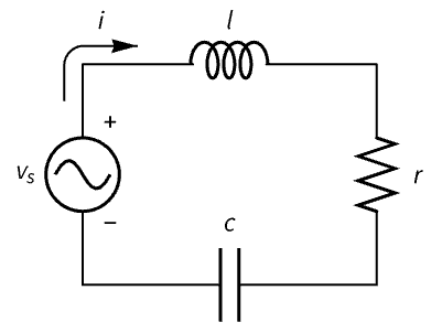
State-space models can represent systems with a mix of differential and algebraic equations. Construct a descriptor state-space model of an RLC circuit from its differential equations and a standard state-space model from its differential equations:

The equations of the individual components:
A descriptor state-space model is obtained because the Kirchhoff equation is algebraic:
The circuit's response to an AC voltage:
Using purely differential equations, a standard state-space model is obtained:
State-space models are used for solving tracking problems. Design an estimator-based tracking controller for a DC motor in the presence of varying torque loads and sensor noise: »
The model specification for the controller design:
Compute a set of estimator gains:
Compute a state-feedback controller:
A noisy signal to simulate the sensor noise:
A signal that simulates a varying torque load:
Simulate the system's response:
Information Systems (1)
Properties & Relations (20)
The eigenvalues of the state matrix are invariant under a similarity transformation:
The transfer function model of state-space models related through a similarity transformation are the same:
The transfer function models are the same:
The controllability property is generally not invariant under a similarity transformation:
The observability property is generally not invariant under a similarity transformation:
The controllable or controllable canonical realization is controllable:
But it is not necessarily observable:
The observable or observable canonical realization is observable:
But it is not necessarily controllable:
The controllable companion and observable companion realizations are duals of each other:
The dual of the controllable companion is the observable companion:
A state-space model's state matrix satisfies its own characteristic polynomial:
The characteristic polynomial:
It satisfies its characteristic polynomial as per the Cayley–Hamilton theorem:
The characteristic polynomial of the state matrix is the denominator of a transfer function model:
The eigenvalues of the state matrix determine the speed of the system's response:
The system response is determined by the exponents:
They are the eigenvalues of the state matrix:
Thus if the state matrix's eigenvalues are negative, the response decays exponentially to zero:
This is because the eigenvalues are all negative:
If the eigenvalues are complex and on the left-hand plane, the response is oscillatory and decays to 0:
Its output response contains sinusoids:
This is because its eigenvalues are a complex pair in the left-hand plane:
The closer the eigenvalue pair is to the negative real axis, the more damped the oscillations:
The second model's eigenvalues are closer to the negative real axis than the first's:
The second model's response is more damped:
The further the complex eigenvalue pair is from the origin, the faster the response:
The second model's eigenvalues are further away from the origin:
The second model's response is faster:
The response of the first model to a unit-step input:
If an eigenvalue pair is on the imaginary axis and the rest are negative, the response has undamped oscillations:
Its output response has undamped sinusoidal expressions:
This is because its eigenvalues include a negative value and a pair on the imaginary axis:
If one of the eigenvalues is zero and the rest are negative, the response will have a nonzero offset:
It converges on a nonzero value:
This is because one of its eigenvalues is zero:
If multiple eigenvalues are zero, the response is unstable and diverges to ∞:
This is because its eigenvalues include more than one zero:
If an eigenvalue is positive, the response is unstable and diverges to ∞:
This is because there is a positive eigenvalue:
If a discrete-time model's eigenvalues are within the unit circle, its response decays to zero:
Its output response decays to zero:
This is because its eigenvalues are within the unit circle:
If any eigenvalue is outside the unit circle, the response is unstable:
Its response is unstable and diverges to ∞:
This is because not all its eigenvalues are inside the unit circle:
Possible Issues (4)
Nonlinearities in a model are approximated:
Use a nonlinear model to prevent the approximation:
Compare the linear and nonlinear step responses:
The state matrix and input matrix must have the same number of rows:
Otherwise, the state-space model cannot be constructed:
The state matrix and output matrix must have the same number of columns:
Otherwise, the state-space model cannot be constructed:
The transmission matrix must have the same number of rows as the output matrix and the same number of columns as the input matrix:
Text
Wolfram Research (2010), StateSpaceModel, Wolfram Language function, https://reference.wolfram.com/language/ref/StateSpaceModel.html (updated 2014).
CMS
Wolfram Language. 2010. "StateSpaceModel." Wolfram Language & System Documentation Center. Wolfram Research. Last Modified 2014. https://reference.wolfram.com/language/ref/StateSpaceModel.html.
APA
Wolfram Language. (2010). StateSpaceModel. Wolfram Language & System Documentation Center. Retrieved from https://reference.wolfram.com/language/ref/StateSpaceModel.html