LinearOptimization[c,{a,b}]
finds a real vector x that minimizes the linear objective ![]() subject to the linear inequality constraints
subject to the linear inequality constraints ![]() .
.
LinearOptimization[c,{a,b},{aeq,beq}]
includes the linear equality constraints ![]() .
.


LinearOptimization
LinearOptimization[f,cons,vars]
finds values of variables vars that minimize the linear objective f subject to linear constraints cons.
LinearOptimization[c,{a,b}]
finds a real vector x that minimizes the linear objective ![]() subject to the linear inequality constraints
subject to the linear inequality constraints ![]() .
.
LinearOptimization[c,{a,b},{aeq,beq}]
includes the linear equality constraints ![]() .
.
LinearOptimization[c,…,{dom1,dom2,…}]
takes xi to be in the domain domi, where domi is Integers or Reals.
LinearOptimization[…,"prop"]
specifies what solution property "prop" should be returned.
Details and Options
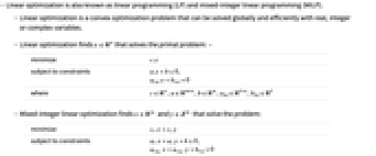


- Linear optimization is also known as linear programming (LP) and mixed-integer linear programming (MILP).
- Linear optimization is a convex optimization problem that can be solved globally and efficiently with real, integer or complex variables.
- Linear optimization finds
 that solves the primal problem: »
 -
minimize 
subject to constraints 
where 
- Mixed-integer linear optimization finds
 and
and  that solve the problem:
 -
minimize 
subject to constraints 
where 
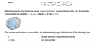
- When the objective function is real valued, LinearOptimization solves problems with
![x in TemplateBox[{}, Complexes]^n](Files/LinearOptimization.en/13.png "x in TemplateBox[{}, Complexes]^n") by internally converting to real variables
by internally converting to real variables  , where
  and
and  .
. - The variable specification vars should be a list with elements giving variables in one of the following forms:
-
v variable with name  and dimensions inferred
v∈Reals real scalar variable v∈Integers integer scalar variable v∈Complexes complex scalar variable v∈ℛ vector variable restricted to the geometric region 
v∈Vectors[n,dom] vector variable in  or
or 
v∈Matrices[{m,n},dom] matrix variable in  or
or 
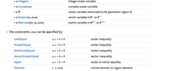
- The constraints cons can be specified by:
-
LessEqual 
scalar inequality GreaterEqual 
scalar inequality VectorLessEqual 
vector inequality VectorGreaterEqual 
vector inequality Equal 
scalar or vector equality Element 
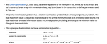
convex domain or region element - With LinearOptimization[f,cons,vars], parameter equations of the form parval, where par is not in vars and val is numerical or an array with numerical values, may be included in the constraints to define parameters used in f or cons.
- The primal minimization problem has a related maximization problem that is the Lagrangian dual problem. The dual maximum value is always less than or equal to the primal minimum value, so it provides a lower bound. The dual maximizer provides information about the primal problem, including sensitivity of the minimum value to changes in the constraints.
- The Lagrangian dual problem for linear optimization is given by: »
-
maximize 
subject to constraints 
where 
- For linear optimization, strong duality always holds, meaning that if there is a solution to the primal minimization problem, then there is a solution to the dual maximization problem, and the dual maximum value is equal to the primal minimum value.
- The possible solution properties "prop" include:
-
"PrimalMinimizer" 
a list of variable values that minimize the objective function "PrimalMinimizerRules" 
values for the variables vars={v1,…} that minimize 
"PrimalMinimizerVector" 
the vector that minimizes 
"PrimalMinimumValue" 
the minimum value 
"DualMaximizer" 
the vector that maximizes 
"DualMaximumValue" 
the dual maximum value "DualityGap" 
the difference between the dual and primal optimal values (0 because of strong duality) "Slack" 
the constraint slack vector "ConstraintSensitivity" 
sensitivity of  to constraint perturbations
"ObjectiveVector" 
the linear objective vector "LinearInequalityConstraints" 
the linear inequality constraint matrix and vector "LinearEqualityConstraints" 
the linear equality constraint matrix and vector {"prop1","prop2",…} several solution properties - The following options can be given:
-
MaxIterations Automatic maximum number of iterations to use Method Automatic the method to use PerformanceGoal $PerformanceGoal aspects of performance to try to optimize Tolerance Automatic the tolerance to use for internal comparisons WorkingPrecision Automatic precision to use in internal computations - The option Method->method may be used to specify the method to use. Available methods include:
-
Automatic choose the method automatically "Simplex" simplex method "RevisedSimplex" revised simplex method "InteriorPoint" interior point method (machine precision only) "CLP" COIN library linear programming (machine precision only) "MOSEK" commercial MOSEK linear optimization solver "Gurobi" commercial Gurobi linear optimization solver "Xpress" commercial Xpress linear optimization solver - With WorkingPrecision->Automatic, the precision is taken automatically from the precision of the input arguments unless a method is specified that only works with machine precision, in which case machine precision is used.
Examples
open all close allBasic Examples (3)
Scope (32)
Basic Uses (16)
Minimize ![]() subject to the constraints
subject to the constraints ![]() :
:
Minimize ![]() subject to the constraints
subject to the constraints ![]() and
and ![]() :
:
Minimize ![]() subject to the constraints
subject to the constraints ![]() and the bounds
and the bounds ![]() :
:
Use VectorLessEqual to express several LessEqual inequality constraints at once:
Use ![]() v<=
v<=![]() to enter the vector inequality in a compact form:
to enter the vector inequality in a compact form:
An equivalent form using scalar inequalities:
Use VectorGreaterEqual to express several GreaterEqual inequality constraints at once:
Use ![]() v>=
v>=![]() to enter the vector inequality in a compact form:
to enter the vector inequality in a compact form:
Use Equal to express several equality constraints at once:
An equivalent form using several scalar equalities:
Specify the constraints using a combination of scalar and vector inequalities:
An equivalent form using scalar inequalities:
Minimize ![]() subject to
subject to ![]() . Use a vector variable
. Use a vector variable ![]() :
:
An equivalent form using scalar variables:
Use vector variables and vector inequalities to specify the problem:
Minimize the function ![]() subject to the constraint
subject to the constraint ![]() :
:
Use Indexed to access components of a vector variable, e.g. ![]() :
:
Use constant parameter equations to specify the coefficients of the objective and constraints:
Use constant parameter equations to specify coefficients of several constraints:
Minimize the function ![]() subject to
subject to ![]() :
:
Use Vectors[n] to specify the dimension of vector variables when needed:
Specify non-negative constraints using NonNegativeReals (![]() ):
):
An equivalent form using vector inequalities:
Specify non-positive constraints using NonPositiveReals (![]() ):
):
An equivalent form using vector inequalities:
Minimize ![]() subject to
subject to ![]() by directly giving the matrix
by directly giving the matrix ![]() and vectors
and vectors ![]() and
and ![]() :
:
Integer Variables (4)
Specify integer domain constraints using Integers:
Specify integer domain constraints on vector variables using Vectors[n,Integers]:
Specify non-negative integer constraints using NonNegativeIntegers (![]() ):
):
An equivalent form using vector inequalities:
Specify non-positive integer constraints using NonPositiveIntegers (![]() ):
):
Complex Variables (2)
Specify complex variables using Complexes:
Minimize a real objective ![]() with complex variables and complex constraints
with complex variables and complex constraints ![]() :
:
Suppose that ![]() ; then expanding out the constraint into real components gives:
; then expanding out the constraint into real components gives:
Solve the problem with real-valued objective and complex variables and constraints:
Primal Model Properties (3)
Minimize the function ![]() subject to the constraints
subject to the constraints ![]() :
:
Get the primal minimizer as a vector:
Obtain the primal minimum value using symbolic inputs:
Extract the matrix-vector inputs of the optimization problem:
Solve using the matrix-vector form:
Recover the symbolic primal value by adding the objective constant:
Find the slack associated with a minimization problem:
Get the primal minimizer and the constraint matrices:
The slack for inequality constraints ![]() is a vector
is a vector ![]() such that
such that ![]() :
:
The slack for the equality constraints ![]() is a vector
is a vector ![]() such that
such that ![]() :
:
Dual Model Properties (3)
The dual problem is to maximize ![]() subject to
subject to ![]() and
and ![]() :
:
The primal minimum value and the dual maximum value coincide because of strong duality:
That is the same as having a duality gap of zero. In general, ![]() at optimal points:
at optimal points:
Construct the dual problem using constraint matrices extracted from the primal problem:
Extract the objective vector and constraint matrices:
The dual problem is to maximize ![]() subject to
subject to ![]() and
and ![]() :
:
Get the dual maximum value directly using solution properties:
Sensitivity Properties (4)
Use "ConstraintSensitivity" to find the change in optimal value due to constraint relaxations:
The first vector is inequality sensitivity and the second is equality sensitivity:
Consider new constraints ![]() where
where ![]() is the relaxation:
is the relaxation:
The expected new optimal value is given by:
Compare to directly solving the relaxed problem:
Each sensitivity is associated with an inequality or equality constraint:
The inequality constraints and their associated sensitivity:
The equality constraints and their associated sensitivity:
The change in optimal value due to constraint relaxation is proportional to the sensitivity value:
Compute the minimal value and constraint sensitivity:
A zero sensitivity will not change the optimal value if the constraint is relaxed:
A negative sensitivity will decrease the optimal value:
A positive sensitivity will increase the optimal value:
The "ConstraintSensitivity" is related to the dual maximizer of the problem:
The inequality sensitivity ![]() satisfies
satisfies ![]() , where
, where ![]() is the dual inequality maximizer:
is the dual inequality maximizer:
The equality sensitivity ![]() satisfies
satisfies ![]() , where
, where ![]() is the dual equality maximizer:
is the dual equality maximizer:
Options (9)
Method (5)
The default method for MachinePrecision input is "CLP":
The default method for arbitrary or infinite WorkingPrecision is "Simplex":
All methods work for MachinePrecision input:
"Simplex" and "RevisedSimplex" can be used for arbitrary- and infinite-precision inputs:
Different methods have different strengths, which is typically problem and implementation dependent:
"Simplex" and "RevisedSimplex" are good for small dense problems:
"InteriorPoint" and "CLP" are good for large sparse problems:
"InteriorPoint" or "CLP" methods may not be able to tell if a problem is infeasible or unbounded:
"Simplex" and "RevisedSimplex" can detect unbounded or infeasible problems:
Different methods may give different results for problems with more than one optimal solution:
"InteriorPoint" may return a solution in the middle of the optimal solution set:
"Simplex" always returns a solution at a corner of the optimal solution set:
Tolerance (2)
A smaller Tolerance setting gives a more precise result:
Specify the constraint matrices:
Find the error between computed and exact minimum value ![]() using different Tolerance settings:
using different Tolerance settings:
Visualize the change in minimum value error with respect to tolerance:
A smaller Tolerance setting gives a more precise answer, but typically takes longer to compute:
WorkingPrecision (2)
LinearOptimization infers the WorkingPrecision to use from the input:
MachinePrecision input gives MachinePrecision output:
LinearOptimization can compute results using higher working precision:
If the specified precision is less than the precision of the input arguments, a message is issued:
Applications (34)
Basic Modeling Transformations (8)
Maximize ![]() subject to
subject to ![]() . Solve a maximization problem by negating the objective function:
. Solve a maximization problem by negating the objective function:
Negate the primal minimum value to get the corresponding maximal value:
Convert ![]() into a linear function using
into a linear function using ![]() and
and ![]() :
:
Convert ![]() into a linear function using
into a linear function using ![]() and
and ![]() :
:
Minimize ![]() subject to the constraints
subject to the constraints ![]() . Convert
. Convert ![]() into a linear function using
into a linear function using ![]() :
:
The problem can also be converted using ![]() :
:
Minimize ![]() subject to the constraints
subject to the constraints ![]() . The constraint can be transformed to
. The constraint can be transformed to ![]() :
:
Minimize ![]() subject to the constraints
subject to the constraints ![]() . The constraint
. The constraint ![]() can be interpreted as
can be interpreted as ![]() . Solve the problem with each constraint:
. Solve the problem with each constraint:
The optimal solution is the minimum of the two solutions:
Minimize ![]() subject to
subject to ![]() , where
, where ![]() is a nondecreasing function, by instead minimizing
is a nondecreasing function, by instead minimizing ![]() . The primal minimizer
. The primal minimizer ![]() will remain the same for both problems. Consider minimizing
will remain the same for both problems. Consider minimizing ![]() subject to
subject to ![]() :
:
The true minimum value can be obtained by applying the function ![]() to the primal minimum value:
to the primal minimum value:
Since ![]() , solve the problem with
, solve the problem with ![]() :
:
The true minimum value can be obtained by applying the function ![]() to the primal minimum value:
to the primal minimum value:
Data-Fitting Problems (4)
Find a robust linear fit to discrete data by minimizing ![]() . Using auxiliary variables
. Using auxiliary variables ![]() , the problem is transformed to minimize
, the problem is transformed to minimize ![]() subject to the constraints
subject to the constraints ![]() , which is a linear optimization problem:
, which is a linear optimization problem:
A plot of the line shows that it is robust to the outliers:
Compare with the fit obtained using LeastSquares:
Find a linear fit by minimizing ![]() such that the line should pass through the first data point:
such that the line should pass through the first data point:
By adding the constraint a〚1〛.xb〚1〛, the line is forced to pass through the first point:
The plot shows that the line passes through the first data point while still maintaining a robust fit:
Find a robust fit to nonlinear discrete data by minimizing ![]() . Generate some noisy data:
. Generate some noisy data:
Fit the data using the bases ![]() . The approximating function will be
. The approximating function will be ![]() :
:
Find the coefficients of the approximating function:
Compare the approximating model with the reference and the least squares fit:
Find a linear fit to discrete data by minimizing ![]() . Since
. Since ![]() , by introducing the scalar auxiliary variable
, by introducing the scalar auxiliary variable ![]() , the problem can be transformed to minimize
, the problem can be transformed to minimize ![]() , subject to the constraints
, subject to the constraints ![]() :
:
The line represents the "best-worst case" fit:
The function Fit can be used directly to compute the coefficients:
Classification Problems (3)
Find a line ![]() that separates two groups of points
that separates two groups of points ![]() and
and ![]() :
:
For separation, set 1 must satisfy ![]() and set 2 must satisfy
and set 2 must satisfy ![]() :
:
Find a quadratic polynomial ![]() that separates two groups of points
that separates two groups of points ![]() and
and ![]() :
:
For separation, set 1 must satisfy ![]() and set 2 must satisfy
and set 2 must satisfy ![]() :
:
The coefficients of the quadratic polynomial are:
Find the minimum-degree polynomial that can separate two sets of points in the plane:
Define a polynomial power function that avoids issues when ![]() or
or ![]() is 0:
is 0:
Define a function that gives a polynomial of degree ![]() with coefficient
with coefficient ![]() as a function of
as a function of ![]() :
:
The variables for a degree ![]() are the coefficients:
are the coefficients:
The constraints enforce separation between set 1 and set 2:
For example, the constraints for quadratics are:
For separation, the only condition is that all the constraints must be satisfied. The objective vector is set to 0:
Manufacturing Problems (3)
Find the mix of products to manufacture that maximizes the profits of a company. The company makes three products. The revenue per unit, cost per unit and maximum capacity are given by:
Each product is made using a combination of four machines. The time a machine spends on each product is:
The profit equals revenue minus cost times the number of units ![]() for product
for product ![]() :
:
Each machine can run at most 2400 minutes per week:
The company makes between zero and the capacity for each product:
The optimal product mix is given by:
The resulting profit is given by:
The breakdown of machining time for each product is:
The same company wants to find out what capacity to change that will have the largest impact on profit. The optimal product mix and profit as formulated previously are given by:
The profit based on the current capacity is:
Extract all the data needed to analyze the impact of the capacity change on profit:
The sensitivity gives the derivative of the profit wrt each of the constraints. Extract the constraints that have any sensitivity at all:
Extract the sensitive constraints from ![]() :
:
If the production capacity for product 3 is increased, there should be an increase in profit:
The resulting increase in profit:
This corresponds exactly to the predicted increase from the sensitivity:
If the production capacity of product 1, product 2 or both is changed, the profit does not increase:
Find the mix of products to manufacture that maximizes the profits of a company. The company makes three products ![]() . The revenue per unit is:
. The revenue per unit is:
The factory is only open for 100 days. It takes ![]() days, respectively, to make each unit:
days, respectively, to make each unit:
Each product contains gold and tin. The total gold and tin available are 30 and 200 units, respectively:
The company incurs a setup cost for each product if that product is manufactured:
Because of the relatively high setup costs, it may be desirable not to manufacture some of the products at all. Let ![]() be a decision variable such that
be a decision variable such that ![]() if product
if product ![]() is manufactured and otherwise
is manufactured and otherwise ![]() . The limit
. The limit ![]() ensures that if
ensures that if ![]() is 0, so is
is 0, so is ![]() , without limiting the size of
, without limiting the size of ![]() more than other constraints do:
more than other constraints do:
Transportation Problems (1)
John Conner has learned that Skynet is planning on attacking five settlements. He needs to deploy soldiers from three base camps to the settlements to meet the threat. The fuel cost to transport one soldier from base camp ![]() to settlement
to settlement ![]() is:
is:
Let ![]() represent the number of soldiers to be shipped from base camp
represent the number of soldiers to be shipped from base camp ![]() to settlement
to settlement ![]() . The cost function to minimize is:
. The cost function to minimize is:
Each base camp needs to distribute a maximum of 100 soldiers between the settlements:
Each settlement needs at least 50 soldiers from a combination of the base camps:
The number of soldiers to be deployed from each base camp to each settlement is:
Optimal Assignment Problems (2)
The Jedi Order is fighting the separatist armies led by Dooku. Dooku and two of his generals, Asajj Ventress and General Grievous, have attacked three outer colonies. The Jedi Order sends three Jedi to assist the outer colonies. Let ![]() be the odds of Jedi
be the odds of Jedi ![]() beating Sith
beating Sith ![]() :
:
Let ![]() be a matrix variable where
be a matrix variable where ![]() is 1 if Jedi
is 1 if Jedi ![]() battles Sith
battles Sith ![]() , and 0 otherwise. The cost function is the expected number of defeats given by
, and 0 otherwise. The cost function is the expected number of defeats given by ![]() and constructed using Inactive[Times]:
and constructed using Inactive[Times]:
Since the outer colonies are far apart, each Jedi may only be assigned to one Sith, and vice versa. Also, since ![]() is 0 or 1, then
is 0 or 1, then ![]() :
:
Find the appropriate Jedi to face the Sith to minimize the chances of defeat:
This means that Obi-Wan Kenobi is sent to General Grievous, Mace Windu is sent to Asajj Ventress and Ki-Adi-Mundi is sent to Dooku. The expected number of defeats is:
Solve a bipartite matching problem between two sets ![]() and
and ![]() that minimizes the total weight:
that minimizes the total weight:
Let ![]() be a matrix variable, where
be a matrix variable, where ![]() is 1 when
is 1 when ![]() is matched to
is matched to ![]() and 0 otherwise. The total weight of the matching is given by
and 0 otherwise. The total weight of the matching is given by ![]() and constructed using Inactive[Times]:
and constructed using Inactive[Times]:
The row and column sums of ![]() need to be 1 and also
need to be 1 and also ![]() :
:
Use LinearOptimization to solve the problem:
The matching permutation may be extracted by converting the matrix ![]() into a graph. Round is used to truncate small values that may occur due to numerical error in some methods:
into a graph. Round is used to truncate small values that may occur due to numerical error in some methods:
Inventory Control Problems (2)
Find the inventory that a retail store must order for a product ![]() per week to minimize cost. Let
per week to minimize cost. Let ![]() be the stock available at the beginning of the week
be the stock available at the beginning of the week ![]() . Let
. Let ![]() be the stock order received from the wholesaler at the beginning of the week
be the stock order received from the wholesaler at the beginning of the week ![]() . The cost to purchase one unit from the wholesaler is $3:
. The cost to purchase one unit from the wholesaler is $3:
The cost of holding excess or negative inventory is $1 per unit. The inventory cost is ![]() , which is not linear but can be represented as
, which is not linear but can be represented as ![]() :
:
The total cost to minimize is ![]() :
:
Let ![]() be the demand at the beginning of the week
be the demand at the beginning of the week ![]() . The demand over a period of 52 weeks is given by
. The demand over a period of 52 weeks is given by ![]() for
for ![]() . The store inventory evolves as
. The store inventory evolves as ![]() :
:
At week 0, there is an existing inventory ![]() units and stock order
units and stock order ![]() units. The store cannot purchase more than 10 units per week from the wholesaler:
units. The store cannot purchase more than 10 units per week from the wholesaler:
Find the optimal inventory to keep in store and order from the wholesaler by minimizing cost:
Here is a plot of inventory, stock order and demand that shows that after week 26, the store does not need to carry any inventory, hence minimizing inventory cost:
Find the inventory that a retail store must order for a product ![]() per week to minimize cost without back orders. Let
per week to minimize cost without back orders. Let ![]() be the stock order received from the wholesaler at the beginning of the week
be the stock order received from the wholesaler at the beginning of the week ![]() . The cost of purchasing one unit from the wholesaler is $3:
. The cost of purchasing one unit from the wholesaler is $3:
The cost of holding excess or negative inventory is $1 per unit:
Let ![]() be the demand at the beginning of the week
be the demand at the beginning of the week ![]() . The demand over a period of 52 weeks is given by
. The demand over a period of 52 weeks is given by ![]() for
for ![]() . The store inventory evolves as
. The store inventory evolves as ![]() :
:
The initial inventory is ![]() units and
units and ![]() units, and the maximum purchase from the wholesaler is 10 units:
units, and the maximum purchase from the wholesaler is 10 units:
The company wants to make sure that there are no back orders, i.e. ![]() :
:
Find the optimal inventory to keep in store and order from the wholesaler by minimizing cost:
This plot shows that in order to avoid back orders, excess inventory must be purchased earlier in the weeks to meet the demand. The store has no inventory costs by weeks 20–21:
Structural Optimization Problems (2)
Minimize the weight of a two-beam truss subject to stress and displacement constraints:

The weight is ![]() , where
, where ![]() is the density, and
is the density, and ![]() and
and ![]() are the cross-sectional areas of bar 1 and bar 2. For this problem, assume
are the cross-sectional areas of bar 1 and bar 2. For this problem, assume ![]() :
:
The forces acting along the axes of bar 1 and bar 2 are:
The stress ![]() , where
, where ![]() is the force acting along the bar, must be less than a specified stress
is the force acting along the bar, must be less than a specified stress ![]() :
:
The displacement at the free node is ![]() . The component of this displacement along the axis of the bar must equal the displacement
. The component of this displacement along the axis of the bar must equal the displacement ![]() , where
, where ![]() is Young's modulus:
is Young's modulus:
The vertical displacement of the free node must be less than a given ![]() :
:
The material being used is aluminium. The design parameters are:
Compute the minimum weight and the optimal cross-sectional areas of the beam:
Find the range of angle and length for which the truss weight does not exceed 180 kg:
Minimize the weight of a two-beam truss subject to stress and displacement constraints, and find the constraints that have a major effect on the design of the truss:

The weight is ![]() , where
, where ![]() is the density, and
is the density, and ![]() and
and ![]() are the cross-sectional areas of bar 1 and bar 2. For this problem, assume
are the cross-sectional areas of bar 1 and bar 2. For this problem, assume ![]() :
:
The constraint due to the forces acting on the bars is:
The material being used is aluminium. The design parameters are:
Minimize the weight of the truss by finding the optimal cross-sectional area ![]() of the bars:
of the bars:
Large constraint sensitivity values indicate a greater influence on the design:
The critical constraint influencing the design is the force constraint ![]() acting on bar 1:
acting on bar 1:
Sequential Linear Optimization (1)
Minimize a nonlinear function ![]() subject to nonlinear constraints
subject to nonlinear constraints ![]() . The minimization can be done by approximating
. The minimization can be done by approximating ![]() as
as ![]() and the constraints as
and the constraints as ![]() as
as ![]() . This leads to a linear minimization problem that can be solved iteratively. Consider a case where
. This leads to a linear minimization problem that can be solved iteratively. Consider a case where ![]() and
and ![]() :
:
The gradients of the minimizing function and constraints are:
The subproblem is to find ![]() by minimizing
by minimizing ![]() subject to
subject to ![]() :
:
Iterate, starting with an initial guess of ![]() . The next iterate is
. The next iterate is ![]() , where
, where ![]() is the step length to ensure that the constraints are always satisfied:
is the step length to ensure that the constraints are always satisfied:
Visualize the convergence of the result. The final result is the green point:
Sudoku Game (3)
Solve the following sudoku puzzle:

Let ![]() be the variable for subsquare
be the variable for subsquare ![]() . Let
. Let ![]() , be the element
, be the element ![]() of vector
of vector ![]() . When
. When ![]() , then
, then ![]() holds the number
holds the number ![]() . Each
. Each ![]() contains only one number, so
contains only one number, so ![]() can contain only one nonzero element, i.e.
can contain only one nonzero element, i.e. ![]() :
:
Each row must contain all the numbers, i.e. ![]() , where
, where ![]() is a nine-dimensional vector of ones:
is a nine-dimensional vector of ones:
Each column must contain all the numbers, i.e. ![]() :
:
Each 3×3 block must contain all the numbers, i.e. ![]() :
:
Collectively, these together make the sudoku constraints for any puzzle:
Convert the known values into constraints. If subsquare ![]() holds number
holds number ![]() , then
, then ![]() :
:
Generate random sudoku boards by randomly specifying the first row. Define a solver function based on the procedure outlined:
Find a feasible solution and compare to the starting board:
Generate sudoku puzzles by randomly generating a board and removing one element at a time. Define a function to solve the sudoku puzzle. If a negative number is specified on the sudoku board, then the function assumes that the number at that position is not allowed:
Generate a random reference sudoku board by randomly specifying the first row of the board:
Specify the minimum number of elements to keep:
Repeatedly remove one randomly selected element from the board at a time until no more elements can be removed without losing the uniqueness of the solution. A removal is tested by solving the sudoku puzzle, with the added condition that the removed element cannot have the removed number. If a feasible solution is found, the number at that position is not unique and the element is retained; otherwise, it is removed from the board:
Visualize the resulting puzzle:
Solve the resulting puzzle and compare with the reference sudoku board:
Graph-Coloring Problem (1)
Find the minimum number of colors needed to color the nodes of a graph such that no two adjacent nodes have the same color. Start with more than a sufficient number of colors for any graph:
Extract the adjacency matrix associated with the graph. Since the matrix is symmetric, only use the upper-triangular part of the matrix:
Let ![]() be a matrix such that
be a matrix such that ![]() if node
if node ![]() is assigned color
is assigned color ![]() . Let
. Let ![]() be a vector such that
be a vector such that ![]() if color
if color ![]() is used in the final set. Each node must be given a color:
is used in the final set. Each node must be given a color:
If two nodes share an edge, then they both cannot be assigned the same color:
If node ![]() is assigned color
is assigned color ![]() , then color
, then color ![]() is used in the final set of colors:
is used in the final set of colors:
The matrix ![]() and the vector
and the vector ![]() are binary variables:
are binary variables:
Solve the graph-coloring problem:
Set-Covering Problems (3)
Find the combination of doctors a hospital emergency room (ER) must keep on call so that the ER can perform a list of procedures. Each doctor can only perform a certain number of procedures:
The cost for keeping each doctor on call is:
Let ![]() be a decision vector such that
be a decision vector such that ![]() if doctor
if doctor ![]() is on call. The objective is to minimize cost:
is on call. The objective is to minimize cost:
At least one doctor must perform procedure ![]() :
:
Find the combination of doctors to keep on call:
Find the minimum number of fire stations that a city containing six districts must build such that there is at least one fire station within 15 minutes of each district. The time required to drive between districts is:
Let ![]() be a decision vector such that
be a decision vector such that ![]() if a fire station is built in district
if a fire station is built in district ![]() . The objective is to minimize the number of fire stations:
. The objective is to minimize the number of fire stations:
At least one fire station must be within 15 minutes of each district:
Find the districts in which a fire station should be built:
Find the minimum number of storage depots a company needs build to distribute to six of its retail stores. The company has selected five possible storage sites. The cost to supply each store from each depot is:
The operating cost and construction cost for each depot is:
Let ![]() be a decision variable such that
be a decision variable such that ![]() if depot
if depot ![]() is built. Let
is built. Let ![]() represent the fraction of goods that depot
represent the fraction of goods that depot ![]() supplies to store
supplies to store ![]() . The objective is to minimize cost:
. The objective is to minimize cost:
Depot ![]() must supply all of its goods to the selected stores:
must supply all of its goods to the selected stores:
Traveling Salesman Problem (1)
Find the path that a salesman should take through ![]() cities such that each city is only visited once and that minimizes the distance. Generate the locations:
cities such that each city is only visited once and that minimizes the distance. Generate the locations:
Let ![]() be the distance between city
be the distance between city ![]() and city
and city ![]() . Let
. Let ![]() be a decision variable such that if
be a decision variable such that if ![]() , the path goes from city
, the path goes from city ![]() to city
to city ![]() . The objective is to minimize distance:
. The objective is to minimize distance:
The salesman can arrive from exactly one city and can depart to exactly one other city:
The salesman cannot arrive at one city and depart to the same city:
The salesman must travel to all the locations in a single tour:
The decision variable is a binary variable and the dummy variable is ![]() :
:
Find the path that minimizes the distance:
Use FindShortestTour to solve the traveling salesman problem much more efficiently:
Properties & Relations (9)
LinearOptimization gives the global minimum of the objective function:
Minimize also gives global exact results for linear optimization problems:
NMinimize can be used to obtain approximate results using global methods:
FindMinimum can be used to obtain approximate results using local methods:
LinearFractionalOptimization uses LinearOptimization for solving problems:
Transform the objective and constraints using ![]() :
:
Obtain the solution to the original problem by applying the inverse transformation:
QuadraticOptimization is a generalization of LinearOptimization:
SecondOrderConeOptimization is a generalization of LinearOptimization:
SemidefiniteOptimization is a generalization of LinearOptimization:
ConicOptimization is a generalization of LinearOptimization:
Possible Issues (6)
Constraints specified using strict inequalities may not be satisfied:
The reason is that LinearOptimization solves ![]() :
:
The minimum value of an empty set or infeasible problem is defined to be ![]() :
:
The minimizer is Indeterminate:
The minimum value for an unbounded set or unbounded problem is ![]() :
:
The minimizer is Indeterminate:
Dual related solution properties for mixed-integer problems may not be available:
Mixed-integer problems can only be solved in machine precision:
Constraints with complex values need to be specified using vector inequalities:
Just using GreaterEqual will not work:
Text
Wolfram Research (2019), LinearOptimization, Wolfram Language function, https://reference.wolfram.com/language/ref/LinearOptimization.html (updated 2020).
CMS
Wolfram Language. 2019. "LinearOptimization." Wolfram Language & System Documentation Center. Wolfram Research. Last Modified 2020. https://reference.wolfram.com/language/ref/LinearOptimization.html.
APA
Wolfram Language. (2019). LinearOptimization. Wolfram Language & System Documentation Center. Retrieved from https://reference.wolfram.com/language/ref/LinearOptimization.html