QuadraticOptimization[{q,c},{a,b}]
finds a vector ![]() that minimizes the quadratic objective
that minimizes the quadratic objective ![]() subject to the linear inequality constraints
subject to the linear inequality constraints ![]() .
.
QuadraticOptimization[{q,c},{a,b},{aeq,beq}]
includes the linear equality constraints ![]() .
.
QuadraticOptimization[{q,c},…,{dom1,dom2,…}]
takes ![]() to be in the domain domi, where domi is Integers or Reals.
to be in the domain domi, where domi is Integers or Reals.


QuadraticOptimization
QuadraticOptimization[f,cons,vars]
finds values of variables vars that minimize the quadratic objective f subject to linear constraints cons.
QuadraticOptimization[{q,c},{a,b}]
finds a vector ![]() that minimizes the quadratic objective
that minimizes the quadratic objective ![]() subject to the linear inequality constraints
subject to the linear inequality constraints ![]() .
.
QuadraticOptimization[{q,c},{a,b},{aeq,beq}]
includes the linear equality constraints ![]() .
.
QuadraticOptimization[{q,c},…,{dom1,dom2,…}]
takes ![]() to be in the domain domi, where domi is Integers or Reals.
to be in the domain domi, where domi is Integers or Reals.
QuadraticOptimization[…,"prop"]
specifies what solution property "prop" should be returned.
Details and Options
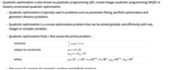


- Quadratic optimization is also known as quadratic programming (QP), mixed-integer quadratic programming (MIQP) or linearly constrained quadratic optimization.
- Quadratic optimization is typically used in problems such as parameter fitting, portfolio optimization and geometric distance problems.
- Quadratic optimization is a convex optimization problem that can be solved globally and efficiently with real, integer or complex variables.
- Quadratic optimization finds
 that solves the primal problem: »
 -
minimize 
subject to constraints 
where 
- The space
 consists of symmetric positive semidefinite matrices.
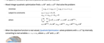
 - Mixed-integer quadratic optimization finds
 and
and  that solve the problem:
 -
minimize 
subject to constraints 
where ![(q_(rr) q_(ri); TemplateBox[{{q, _, {(, {r, , i}, )}}}, Transpose] q_(ii)) in S_+^n,c_r in R^(n_r),c_i in R^(n_i),a_r in R^(mxn_r),a_i in R^(mxn_i),b in R^m,a_(eq_r) in R^(kxn_r),a_(eq_i) in R^(kxn_i)b_(eq) in R^k](Files/QuadraticOptimization.en/15.png "(q_(rr) q_(ri); TemplateBox[{{q, _, {(, {r, , i}, )}}}, Transpose] q_(ii)) in S_+^n,c_r in R^(n_r),c_i in R^(n_i),a_r in R^(mxn_r),a_i in R^(mxn_i),b in R^m,a_(eq_r) in R^(kxn_r),a_(eq_i) in R^(kxn_i)b_(eq) in R^k")
- When the objective function is real valued, QuadraticOptimization solves problems with
![x in TemplateBox[{}, Complexes]^n](Files/QuadraticOptimization.en/16.png "x in TemplateBox[{}, Complexes]^n") by internally converting to real variables
by internally converting to real variables  , where
  and
and  .
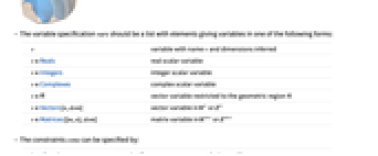
. - The variable specification vars should be a list with elements giving variables in one of the following forms:
-
v variable with name  and dimensions inferred
v∈Reals real scalar variable v∈Integers integer scalar variable v∈Complexes complex scalar variable v∈ℛ vector variable restricted to the geometric region 
v∈Vectors[n,dom] vector variable in  or
or 
v∈Matrices[{m,n},dom] matrix variable in  or
or 
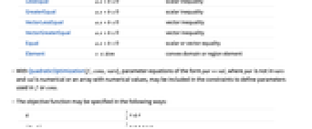
- The constraints cons can be specified by:
-
LessEqual 
scalar inequality GreaterEqual 
scalar inequality VectorLessEqual 
vector inequality VectorGreaterEqual 
vector inequality Equal 
scalar or vector equality Element 
convex domain or region element - With QuadraticOptimization[f,cons,vars], parameter equations of the form parval, where par is not in vars and val is numerical or an array with numerical values, may be included in the constraints to define parameters used in f or cons.
- The objective function may be specified in the following ways:
-
q 
{q,c} 
},c}")
![1/2(q_f.x).(q_f.x)+c.x=1/2(x.TemplateBox[{{q, _, f}}, Transpose]).(q_f.x)+c.x](Files/QuadraticOptimization.en/36.png "1/2(q_f.x).(q_f.x)+c.x=1/2(x.TemplateBox[{{q, _, f}}, Transpose]).(q_f.x)+c.x")
,c_(f)},c}")
![1/2(c_f+q_f.x).(c_f+q_f.x)+c.x=1/2(x.TemplateBox[{{q, _, f}}, Transpose]+c_f).(q_f.x+c_f)+c.x](Files/QuadraticOptimization.en/38.png "1/2(c_f+q_f.x).(c_f+q_f.x)+c.x=1/2(x.TemplateBox[{{q, _, f}}, Transpose]+c_f).(q_f.x+c_f)+c.x")
- In the factored form,
 and
and  .
. - The primal minimization problem has a related maximization problem that is the Lagrangian dual problem. The dual maximum value is always less than or equal to the primal minimum value, so it provides a lower bound. The dual maximizer provides information about the primal problem, including sensitivity of the minimum value to changes in the constraints.
- The Lagrangian dual problem for quadratic optimization with objective
 is given by: »
 -
maximize 
subject to constraints 
where 
- With a factored quadratic objective
![1/2(x.TemplateBox[{{q, _, f}}, Transpose]+c_f).(q_f.x+c_f)+c.x](Files/QuadraticOptimization.en/45.png "1/2(x.TemplateBox[{{q, _, f}}, Transpose]+c_f).(q_f.x+c_f)+c.x") , the dual problem may also be expressed as:
, the dual problem may also be expressed as: -
maximize 
subject to constraints 
where 
- The relationship between the factored dual vector
 and the unfactored dual vector
  is
is  .
. - For quadratic optimization, strong duality holds if
 is positive semidefinite. This means that if there is a solution to the primal minimization problem, then there is a solution to the dual maximization problem, and the dual maximum value is equal to the primal minimum value.
 - The possible solution properties "prop" include:
-
"PrimalMinimizer" 
a list of variable values that minimizes the objective function "PrimalMinimizerRules" 
values for the variables vars={v1,…} that minimizes 
"PrimalMinimizerVector" 
the vector that minimizes 
"PrimalMinimumValue" 
the minimum value 
"DualMaximizer" 
vectors that maximize 
"DualMaximumValue" 
the dual maximum value "DualityGap" 
the difference between the dual and primal optimal values (0 because of strong duality) "Slack" 
the constraint slack vector "ConstraintSensitivity" 
sensitivity of  to constraint perturbations
"ObjectiveMatrix" 
the quadratic objective matrix "ObjectiveVector" 
the linear objective vector "FactoredObjectiveMatrix" 
the matrix in the factored objective form "FactoredObjectiveVector" 
the vector in the factored objective form "LinearInequalityConstraints" 
the linear inequality constraint matrix and vector "LinearEqualityConstraints" 
the linear equality constraint matrix and vector {"prop1","prop2",…} several solution properties - The dual maximizer component
 is a function of
  and
and  , given by
  .
. - The following options may be given:
-
MaxIterations Automatic maximum number of iterations to use Method Automatic the method to use PerformanceGoal $PerformanceGoal aspects of performance to try to optimize Tolerance Automatic the tolerance to use for internal comparisons WorkingPrecision MachinePrecision precision to use in internal computations - The option Method->method may be used to specify the method to use. Available methods include:
-
Automatic choose the method automatically "COIN" COIN quadratic programming solver "SCS" SCS splitting conic solver "OSQP" OSQP operator splitting solver for quadratic problems "CSDP" CSDP semidefinite optimization solver "DSDP" DSDP semidefinite optimization solver "PolyhedralApproximation" objective epigraph is approximated using polyhedra "MOSEK" commercial MOSEK convex optimization solver "Gurobi" commercial Gurobi linear and quadratic optimization solver "Xpress" commercial Xpress linear and quadratic optimization solver
Examples
open all close allBasic Examples (3)
Minimize ![]() subject to the constraint
subject to the constraint ![]() :
:
The optimal point lies in a region defined by the constraints and where ![]() is smallest:
is smallest:
Minimize ![]() subject to the equality constraint
subject to the equality constraint ![]() and the inequality constraints
and the inequality constraints ![]() :
:
Define objective as ![]() and constraints as
and constraints as ![]() and
and ![]() :
:
Solve using matrix-vector inputs:
The optimal point lies where a level curve of ![]() is tangent to the equality constraint:
is tangent to the equality constraint:
Scope (26)
Basic Uses (8)
Minimize ![]() subject to the constraints
subject to the constraints ![]() :
:
Get the minimizing value using solution property "PrimalMinimumValue":
Minimize ![]() subject to the constraint
subject to the constraint ![]() :
:
Get the minimizing value and minimizing vector using solution property:
Minimize ![]() subject to the constraint
subject to the constraint ![]() :
:
Define the objective as ![]() and constraints as
and constraints as ![]() :
:
Solve using matrix-vector inputs:
Minimize ![]() subject to the equality constraint
subject to the equality constraint ![]() and the inequality constraint
and the inequality constraint ![]() :
:
Define objective as ![]() and constraints as
and constraints as ![]() and
and ![]() :
:
Solve using matrix-vector inputs:
Minimize ![]() subject to the constraints
subject to the constraints ![]() :
:
Define the objective as ![]() and constraints as
and constraints as ![]() :
:
Solve using matrix-vector inputs:
Minimize ![]() subject to the constraints
subject to the constraints ![]() :
:
Specify constraints ![]() using VectorGreaterEqual () and VectorLessEqual ():
using VectorGreaterEqual () and VectorLessEqual ():
Minimize ![]() subject to
subject to ![]() . Use a vector variable and constant parameter equations:
. Use a vector variable and constant parameter equations:
Minimize ![]() subject to
subject to ![]() . Use NonNegativeReals to specify the constraint
. Use NonNegativeReals to specify the constraint ![]() :
:
Integer Variables (4)
Specify integer domain constraints using Integers:
Specify integer domain constraints on vector variables using Vectors[n,Integers]:
Specify non-negative integer domain constraints using NonNegativeIntegers (![]() ):
):
Specify non-positive integer constraints using NonPositiveIntegers (![]() ):
):
Complex Variables (3)
Specify complex variables using Complexes:
Use a Hermitian matrix ![]() in the objective
in the objective ![]() with real-valued variables:
with real-valued variables:
Use a Hermitian matrix ![]() in the objective
in the objective ![]() and complex variables:
and complex variables:
Primal Model Properties (4)
Minimize ![]() subject to the constraint
subject to the constraint ![]() :
:
Get vector output using "PrimalMinimizer":
Get the rule-based result using "PrimalMinimizerRules":
Get the minimizing value of the optimization using "PrimalMinimumValue":
Obtain the primal minimum value using symbolic inputs:
Extract the matrix-vector inputs of the optimization problem:
Solve using the matrix-vector form:
Recover the symbolic primal value by adding the objective constant:
Find the slack for inequalities and equalities associated with a minimization problem:
Get the minimum value and the constraint matrices:
The slack for inequality constraints ![]() is a vector
is a vector ![]() such that
such that ![]() :
:
The slack for the equality constraints ![]() is a vector
is a vector ![]() such that
such that ![]() :
:
Dual Model Properties (3)
The dual problem is to maximize ![]() subject to
subject to ![]() :
:
The primal minimum value and the dual maximum value coincide because of strong duality:
So it has a duality gap of zero. In general, ![]() at optimal points:
at optimal points:
Construct the dual problem using constraint matrices extracted from the primal problem:
Extract the objective and constraint matrices and vectors:
The dual problem is to maximize ![]() subject to
subject to ![]() :
:
Get the dual maximum value directly using solution properties:
Sensitivity Properties (4)
Use "ConstraintSensitivity" to find the change in optimal value due to constraint relaxations:
The first vector is inequality sensitivity and the second is equality sensitivity:
Consider new constraints ![]() where
where ![]() is the relaxation:
is the relaxation:
The approximate new optimal value is given by:
Compare to directly solving the relaxed problem:
Each sensitivity is associated with an inequality or equality constraint:
The inequality constraints and their associated sensitivity:
The equality constraints and their associated sensitivity:
The change in optimal value due to constraint relaxation is proportional to the sensitivity value:
Compute the minimal value and constraint sensitivity:
A zero sensitivity will not change the optimal value if the constraint is relaxed:
A negative sensitivity will decrease the optimal value:
A positive sensitivity will increase the optimal value:
The "ConstraintSensitivity" is related to the dual maximizer of the problem:
The inequality sensitivity ![]() satisfies
satisfies ![]() , where
, where ![]() is the dual inequality maximizer:
is the dual inequality maximizer:
The equality sensitivity ![]() satisfies
satisfies ![]() , where
, where ![]() is the dual equality maximizer:
is the dual equality maximizer:
Options (12)
Method (5)
The method "COIN" uses the COIN library:
"CSDP" and "DSDP" reduce to semidefinite optimization:
"SCS" reduces to conic optimization:
"PolyhedralApproximation" approximates the objective using linear constraints:
For least-squares-type quadratic problems, "CSDP" and "DSDP" will be slower than "COIN" or "SCS":
Solve the least-squares problem using method "COIN":
Solve the problem using method "CSDP":
For least-squares-type quadratic problems, "CSDP","DSDP" and "PolyhedralApproximation" will be slower than "COIN" or "SCS":
Solve the least-squares problem using method "COIN":
Solve the problem using method "CSDP":
Solve the problem using method "PolyhedralApproximation":
Different methods may give different results for problems with more than one optimal solution:
Minimizing a concave function can be done only using Method"COIN":
Other methods cannot be used because they require the factorization of the objective matrix:
PerformanceGoal (1)
Tolerance (2)
A smaller Tolerance setting gives a more precise result:
Find the error between computed and exact minimum value using different Tolerance settings:
Visualize the change in minimum value error with respect to tolerance:
A smaller Tolerance setting gives a more precise answer, but typically takes longer to compute:
WorkingPrecision (4)
MachinePrecision is the default for the WorkingPrecision option in QuadraticOptimization:
With WorkingPrecisionAutomatic, QuadraticOptimization infers the precision to use from input:
QuadraticOptimization can compute results using arbitrary-precision numbers:
If the specified precision is less than the precision of the input arguments, a message is issued:
If a high-precision result cannot be computed, a message is issued and a MachinePrecision result is returned:
Applications (29)
Basic Modeling Transformations (7)
Maximize ![]() subject to
subject to ![]() . Solve the maximization problem by negating the objective function:
. Solve the maximization problem by negating the objective function:
Negate the primal minimum value to get the corresponding maximum value:
Minimize ![]() by converting the objective function into
by converting the objective function into ![]() :
:
Construct the objective function by expanding ![]() :
:
Since QuadraticOptimization minimizes ![]() , the matrix is multiplied by 2:
, the matrix is multiplied by 2:
The minimal value of the original function is recovered as ![]() :
:
QuadraticOptimization directly performs this transformation. Construct the objective function using Inactive to avoid threading:
Minimize ![]() subject to the constraints
subject to the constraints ![]() . Transform the objective function to
. Transform the objective function to ![]() and solve the problem:
and solve the problem:
Recover the original minimum value using transformation ![]() :
:
Minimize ![]() subject to the constraints
subject to the constraints ![]() . The constraint can be transformed to
. The constraint can be transformed to ![]() :
:
Minimize ![]() subject to the constraints
subject to the constraints ![]() . The constraint
. The constraint ![]() can be interpreted as
can be interpreted as ![]() . Solve the problem with each constraint:
. Solve the problem with each constraint:
The optimal solution is the minimum of the two solutions:
Minimize ![]() subject to
subject to ![]() , where
, where ![]() is a non-decreasing function, by instead minimizing
is a non-decreasing function, by instead minimizing ![]() . The primal minimizer
. The primal minimizer ![]() will remain the same for both problems. Consider minimizing
will remain the same for both problems. Consider minimizing ![]() subject to
subject to ![]() :
:
The true minimum value can be obtained by applying the function ![]() to the primal minimum value:
to the primal minimum value:
Since ![]() , the solution is the true solution only if the primal minimum value is greater than 0. The true minimum value can be obtained by applying the function
, the solution is the true solution only if the primal minimum value is greater than 0. The true minimum value can be obtained by applying the function ![]() to the primal minimum value:
to the primal minimum value:
Data-Fitting Problems (7)
Find a linear fit to discrete data by minimizing ![]() :
:
Construct the factored quadratic matrix using DesignMatrix:
Find the coefficients of the line:
Find a quadratic fit to discrete data by minimizing ![]() :
:
Construct the factored quadratic matrix using DesignMatrix:
Find the coefficients of the quadratic curve:
Fit a quadratic curve discrete data such that the first and last points of the data lie on the curve:
Construct the factored quadratic matrix using DesignMatrix:
The two equality constraints are:
Find the coefficients of the line:
Find an interpolating function to noisy data using bases ![]() :
:
The interpolating function will be ![]() :
:
Find the coefficients of the interpolating function:
Minimize ![]() subject to the constraints
subject to the constraints ![]() :
:
Compare with the unconstrained minimum of ![]() :
:
Cardinality constrained least squares: minimize ![]() such that
such that ![]() has at most
has at most ![]() nonzero elements:
nonzero elements:
Let ![]() be a decision vector such that if
be a decision vector such that if ![]() , then
, then ![]() is nonzero. The decision constraints are:
is nonzero. The decision constraints are:
To model constraint ![]() when
when ![]() , chose a large constant
, chose a large constant ![]() such that
such that ![]() :
:
Solve the cardinality constrained least-squares problem:
The subset selection can also be done more efficiently with Fit using ![]() regularization. First, find the range of regularization parameters that uses at most
regularization. First, find the range of regularization parameters that uses at most ![]() basis functions:
basis functions:
Find the nonzero terms in the ![]() regularized fit:
regularized fit:
Find the fit with just these basis terms:
Find the best subset of functions from a candidate set of functions to approximate given data:
The approximating function will be ![]() :
:
A maximum of 5 basis functions is to be used in the final approximation:
The coefficients associated with functions that are not chosen must be zero:
Classification Problems (2)
Find a plane ![]() that separates two groups of 3D points
that separates two groups of 3D points ![]() and
and ![]() :
:
For separation, set 1 must satisfy ![]() and set 2 must satisfy
and set 2 must satisfy ![]() . Find the hyperplane by minimizing
. Find the hyperplane by minimizing ![]() :
:
The distance between the planes ![]() and
and ![]() is
is ![]() :
:
The plane separating the two groups of points is:
Plot the plane separating the two datasets:
Find a quadratic polynomial that separates two groups of 3D points ![]() and
and ![]() :
:
Construct the quadratic polynomial data matrices for the two sets using DesignMatrix:
For separation, set 1 must satisfy ![]() and set 2 must satisfy
and set 2 must satisfy ![]() . Find the separating surface by minimizing
. Find the separating surface by minimizing ![]() :
:
Geometric Problems (3)
Find a point ![]() closest to the point
closest to the point ![]() that lies on the planes
that lies on the planes ![]() and
and ![]() :
:
Find the point closest to ![]() by minimizing
by minimizing ![]() . Use Inactive Plus when constructing the objective:
. Use Inactive Plus when constructing the objective:
Find the distance between two convex polyhedra:
Show the nearest points with the line connecting them:
Find the radius ![]() and center
and center ![]() of a minimal enclosing ball that encompasses a given region:
of a minimal enclosing ball that encompasses a given region:
The original minimization problem is to minimize ![]() subject to
subject to ![]() . The dual of this problem is to maximize
. The dual of this problem is to maximize ![]() subject to
subject to ![]() :
:
Solve the dual maximization problem:
The center of the minimal enclosing ball is ![]() :
:
The radius of the minimal enclosing ball is Sqrt of the maximum value:
The minimal enclosing ball can be found efficiently using BoundingRegion:
Investment Problems (3)
Find the number of stocks to buy from four stocks, such that a minimum $1000 dividend is received and risk is minimized. The expected return value and the covariance matrix ![]() associated with the stocks are:
associated with the stocks are:
The unit price for the four stocks is $1. Each stock can be allocated a maximum of $2500:
The investment must yield a minimum of $1000:
A negative stock cannot be bought:
The total amount to spend on each stock is found by minimizing the risk given by ![]() :
:
The total investment to get a minimum of $1000 is:
Find the number of stocks to buy from four stocks, with an option to short-sell such that a minimum dividend of $1000 is received and the overall risk is minimized:
The capital constraint and return on investment constraints are:
A short-sale option allows the stock to be sold. The optimal number of stocks to buy/short-sell is found by minimizing the risk given by the objective ![]() :
:
The second stock can be short-sold. The total investment to get a minimum of $1000 due to the short-selling is:
Without short-selling, the initial investment will be significantly greater:
Find the best combination of six stocks to invest in out of a possible 20 candidate stocks, so as to maximize return while minimizing risk:
Let ![]() be the percentage of total investment made in stock
be the percentage of total investment made in stock ![]() . The return is given by
. The return is given by ![]() , where
, where ![]() is a vector of the expected return value of each individual stock:
is a vector of the expected return value of each individual stock:
Let ![]() be a decision vector such that if
be a decision vector such that if ![]() , then that stock is bought. Six stocks have to be chosen:
, then that stock is bought. Six stocks have to be chosen:
The percentage of investment ![]() must be greater than 0 and must add to 1:
must be greater than 0 and must add to 1:
Find the optimal combination of stocks that minimizes the risk given by ![]() and maximizes return:
and maximizes return:
The optimal combination of stocks is:
The percentages of investment to put into the respective stocks are:
Portfolio Optimization (1)
Find the distribution of capital to invest in six stocks to maximize return while minimizing risk:
Let ![]() be the percentage of total investment made in stock
be the percentage of total investment made in stock ![]() . The return is given by
. The return is given by ![]() , where
, where ![]() is a vector of expected return value of each individual stock:
is a vector of expected return value of each individual stock:
The risk is given by ![]() , and
, and ![]() is a risk-aversion parameter:
is a risk-aversion parameter:
The objective is to maximize return while minimizing risk for a specified risk-aversion parameter ![]() :
:
The percentage of investment ![]() must be greater than 0 and must add to 1:
must be greater than 0 and must add to 1:
Compute the returns and corresponding risk for a range of risk-aversion parameters:
The optimal ![]() over a range of
over a range of ![]() gives an upper-bound envelope on the tradeoff between return and risk:
gives an upper-bound envelope on the tradeoff between return and risk:
Compute the percentage of investment ![]() for a specified number of risk-aversion parameters:
for a specified number of risk-aversion parameters:
Increasing the risk-aversion parameter ![]() leads to stock diversification to reduce the risk:
leads to stock diversification to reduce the risk:
Increasing the risk-aversion parameter ![]() leads to a reduced expected return on investment:
leads to a reduced expected return on investment:
Trajectory Optimization Problems (2)
Minimize ![]() subject to
subject to ![]() . The minimizing function integral can be approximated using the trapezoidal rule. The discretized objective function will be
. The minimizing function integral can be approximated using the trapezoidal rule. The discretized objective function will be ![]() :
:
The constraint ![]() can be discretized using finite differences:
can be discretized using finite differences:
The constraints ![]() can be represented using the Indexed function:
can be represented using the Indexed function:
The constraints ![]() can be discretized using finite differences, and only the first and last rows are used:
can be discretized using finite differences, and only the first and last rows are used:
Solve the discretized trajectory problem:
Convert the discretized result into an InterpolatingFunction:
Compare the result with the analytic solution:
Find the shortest path between two points while avoiding obstacles. Specify the obstacle:
Extract the half-spaces that form the convex obstacle:
Specify the start and end points of the path:
The path can be discretized using ![]() points. Let
points. Let ![]() represent the position vector:
represent the position vector:
The objective is to minimize ![]() . Let
. Let ![]() . The objective is transformed to
. The objective is transformed to ![]() :
:
Specify the end point constraints:
The distance between any two subsequent points should not be too large:
A point ![]() is outside the object if at least one element of
is outside the object if at least one element of ![]() is less than zero. To enforce this constraint, let
is less than zero. To enforce this constraint, let ![]() be a decision vector and
be a decision vector and ![]() be the
be the ![]()
![]() element of
element of ![]() such that
such that ![]() , then
, then ![]() and
and ![]() is large enough such that
is large enough such that ![]() :
:
Find the minimum distance path around the obstacle:
To avoid potential crossings at the edges, the region can be inflated and the problem solved again:
Optimal Control Problems (2)
The integral can be discretized using the trapezoidal method:
The time derivative in ![]() is discretized using finite differences:
is discretized using finite differences:
The end-condition constraints ![]() can be specified using Indexed:
can be specified using Indexed:
Solve the discretized problem:
Convert the discretized result into InterpolatingFunction:
Minimize ![]() subject to
subject to ![]() and
and ![]() and
and ![]() on the control variable:
on the control variable:
The integral can be discretized using the trapezoidal method:
The time derivative in ![]() is discretized using finite differences:
is discretized using finite differences:
The end-condition constraints ![]() can be specified using Indexed:
can be specified using Indexed:
The constraint on the control variable ![]() is:
is:
Solve the discretized problem:
Convert the discretized result into InterpolatingFunction:
Sequential Quadratic Optimization (2)
Minimize a nonlinear function ![]() subject to nonlinear constraints
subject to nonlinear constraints ![]() . The minimization can be done by approximating
. The minimization can be done by approximating ![]() as
as ![]() and the constraints as
and the constraints as ![]() as
as ![]() . This leads to a quadratic minimization problem that can be solved iteratively. Consider a case where
. This leads to a quadratic minimization problem that can be solved iteratively. Consider a case where ![]() and
and ![]() :
:
The gradient and Hessian of the minimizing function are:
The gradient of the constraints is:
The subproblem is to find ![]() by minimizing
by minimizing ![]() subject to
subject to ![]() :
:
Iterate starting with an initial guess of ![]() . The next iterate is
. The next iterate is ![]() , where
, where ![]() is the step length to ensure that the constraints are always satisfied:
is the step length to ensure that the constraints are always satisfied:
Visualize the convergence of the result. The final result is the green point:
The gradient and Hessian of the minimizing function are:
The gradient of the constraints is:
The subproblem is to minimize ![]() , subject to
, subject to ![]() and
and ![]() :
:
Iterate starting with the initial guess ![]() :
:
Visualize the convergence of the result. The final result is the green point:
Properties & Relations (9)
QuadraticOptimization gives the global minimum of the objective function:
Visualize the objective function:
The minimizer can be in the interior or at the boundary of the feasible region:
Minimize gives global exact results for quadratic optimization problems:
NMinimize can be used to obtain approximate results using global methods:
FindMinimum can be used to obtain approximate results using local methods:
LinearOptimization is a special case of QuadraticOptimization:
In matrix-vector form, the quadratic term is set to 0:
SecondOrderConeOptimization is a generalization of QuadraticOptimization:
Use auxiliary variable ![]() and minimize
and minimize ![]() with additional constraint
with additional constraint ![]() :
:
SemidefiniteOptimization is a generalization of QuadraticOptimization:
Use auxiliary variable ![]() and minimize
and minimize ![]() with additional constraint
with additional constraint ![]() :
:
ConicOptimization is a generalization of QuadraticOptimization:
Use auxiliary variable ![]() and minimize
and minimize ![]() with additional constraint
with additional constraint ![]() :
:
Possible Issues (6)
Constraints specified using strict inequalities may not be satisfied for certain methods:
The reason is that QuadraticOptimization solves ![]() :
:
The minimum value of an empty set or infeasible problem is defined to be ![]() :
:
The minimizer is Indeterminate:
The minimum value for an unbounded set or unbounded problem is ![]() :
:
The minimizer is Indeterminate:
Certain solution properties are not available for symbolic input:
Dual related solution properties for mixed-integer problems may not be available:
Constraints with complex values need to be specified using vector inequalities:
Just using GreaterEqual will not work:
Text
Wolfram Research (2019), QuadraticOptimization, Wolfram Language function, https://reference.wolfram.com/language/ref/QuadraticOptimization.html (updated 2020).
CMS
Wolfram Language. 2019. "QuadraticOptimization." Wolfram Language & System Documentation Center. Wolfram Research. Last Modified 2020. https://reference.wolfram.com/language/ref/QuadraticOptimization.html.
APA
Wolfram Language. (2019). QuadraticOptimization. Wolfram Language & System Documentation Center. Retrieved from https://reference.wolfram.com/language/ref/QuadraticOptimization.html